Many-Worlds Interpretation vs Huayan Buddhism’s “Infinite Interpenetration” — Endless Parallel Universes
Series: Quantum Mechanics Meets Eastern Philosophy #06/12 | Reading time: 35-40 min | Python (NumPy, Matplotlib)
Author: Wina @ Code & Cogito
The Forgotten Genius
- Princeton University.
A 27-year-old doctoral student named Hugh Everett III submitted his dissertation to his advisor, John Wheeler.
The title: “Relative State” Formulation of Quantum Mechanics.
Its central claim could be stated in a single sentence:
The wave function never collapses.
What does that imply?
It means Schrodinger’s cat is not “either dead or alive once you open the box.”
Instead:
– When you open the box, the universe splits into two worlds
– In World A, the cat is dead
– In World B, the cat is alive
– Both worlds are equally real, but neither can observe the other
Wheeler read the dissertation and was stunned.
“This… is crazy,” he said.
But he couldn’t find a logical flaw.
Everett held firm: “This is the natural consequence of the quantum mechanical equations. No extra assumptions. No mysterious ‘collapse’ process. The wave function simply evolves according to the Schrodinger equation. That’s it.”
In 1957, the paper was published in Reviews of Modern Physics.
The physics community’s response: total silence.
When Niels Bohr heard about it, he reportedly dismissed it: “This is nonsense!”
Heartbroken, Everett left physics entirely and took a job at the Pentagon.
In 1973, physicist Bryce DeWitt rediscovered the theory and gave it a far catchier name:
“The Many-Worlds Interpretation” (MWI)
In 1982, Everett died in his sleep at the age of 51.
His daughter Elizabeth later took her own life. Her note read:
“I’m going to a parallel universe to find my father.”
Today, the Many-Worlds Interpretation is one of the most popular interpretations of quantum mechanics.
A 2022 survey of physicists found:
– 18% support the Copenhagen interpretation
– 42% support the Many-Worlds Interpretation
Everett’s “crazy” idea is going mainstream.
The Many-Worlds Interpretation: The Wave Function Never Collapses
The Core Claim
The Many-Worlds Interpretation rests on a single core claim:
The universal wave function evolves according to the Schrodinger equation and never collapses.
The consequences of this claim are staggering:
- Every measurement splits the universe
- It’s not “the wave function collapses to one result”
-
It’s “the universe branches into multiple worlds, each corresponding to a possible outcome”
-
All possible outcomes actually occur
- Schrodinger’s cat: the cat is both dead and alive — in different worlds
-
Double-slit experiment: the photon takes all paths — in different worlds
-
“You” exist in countless worlds
- Each world contains a version of “you”
- Each version has different experiences
-
But each version believes it is the only one
-
Worlds cannot communicate
- After branching, worlds cannot observe each other
- Decoherence rapidly makes branches independent
- You can never know about the “you” in other worlds
Mathematical Expression
Suppose a system has two possible states: |0⟩ and |1⟩.
Initial state: |psi⟩ = alpha|0⟩ + beta|1⟩ (superposition)
The Copenhagen interpretation says:
– After measurement, the wave function collapses
– Probability |alpha|^2 of getting |0⟩
– Probability |beta|^2 of getting |1⟩
– Collapse is instantaneous and non-unitary (violating the Schrodinger equation)
The Many-Worlds interpretation says:
– After measurement, the universe splits
– World A: the system is in |0⟩, the observer sees “0”
– World B: the system is in |1⟩, the observer sees “1”
– Total wave function: |Psi⟩ = alpha|0⟩|observer sees 0⟩ + beta|1⟩|observer sees 1⟩
– This is the natural result of the Schrodinger equation — no “collapse” needed
Advantages
The Many-Worlds Interpretation has several compelling advantages:
- Mathematical simplicity
- Only requires the Schrodinger equation
- No additional “collapse” postulate needed
-
Wave function evolution is always unitary
-
Solves the measurement problem
- Copenhagen: What counts as a “measurement”? When does collapse happen?
-
Many-Worlds: There is no “measurement” — only interactions and decoherence
-
Compatible with quantum cosmology
- The universe as a whole has no “external observer”
- The wave function encompasses the entire universe
-
Many-Worlds applies naturally
-
Falsifiability (in principle)
- If we could observe “world merging” (the reverse of decoherence)
- That would falsify the Many-Worlds Interpretation
- Though in practice this is extraordinarily difficult
Disadvantages
The Many-Worlds Interpretation also faces serious challenges:
- Ontological explosion
- The universe constantly splits, producing countless worlds
- Each world “really” exists
-
Isn’t this absurdly extravagant?
-
The origin of probability
- If all outcomes occur, why do probabilities exist?
- Why do we observe |alpha|^2 and |beta|^2?
-
This is the core puzzle of MWI (the “Born rule problem”)
-
Unverifiable
- We can never observe other worlds
-
Is this a scientific theory? Or philosophical speculation?
-
Philosophically unsettling
- Countless versions of “me” exist?
- What happened to my uniqueness?
- Does free will still mean anything?
Huayan Buddhism’s “Infinite Interpenetration”: Boundless Realms
In the 7th century, during China’s Tang Dynasty, a school of Buddhist philosophy emerged that would develop one of the most extraordinary visions of reality ever conceived. Huayan Buddhism — named after the Avatamsaka Sutra (the “Flower Garland Sutra”) — proposed a universe of infinite mutual containment.
Chengguan (738-839), the fourth patriarch of the Huayan school, summarized its core insight:
“Dharmadhatu arising through interdependence — layered without limit.”
For readers less familiar with Buddhist terminology: Dharmadhatu refers to the totality of all phenomena, the entire realm of reality. “Arising through interdependence” means that nothing exists independently — everything emerges through its relationships with everything else.
The Avatamsaka Sutra describes this vision poetically:
“Within a single mote of dust, worlds as numerous as dust motes;
In each of these worlds, Buddhas beyond reckoning;
Each Buddha dwelling among vast assemblies;
I see them all ceaselessly teaching the path.”
In plain language:
– A single particle of dust contains numberless worlds
– Each world contains numberless Buddhas (awakened beings)
– Each is actively teaching
– The layers of reality are infinite
What does this really mean?
Ten Layers of Worlds
Huayan philosophy describes reality as having “ten layers” of worlds:
- This world – our own realm of experience
- Other worlds – countless other realms
- One Buddha-land – a single Buddha’s realm
- Ten Buddha-lands – the ten directions
- A hundred Buddha-lands
- A thousand Buddha-lands
- Ten thousand Buddha-lands
- A hundred million Buddha-lands
- Inconceivably many Buddha-lands
- Buddha-lands within each dust mote – each particle contains infinite worlds
The key insight: each level contains the entirety of all other levels.
This forms a structure of infinite recursion.
“One Is All, All Is One” — Taken to Its Logical Extreme
The foundational principle of Huayan philosophy is “one is all, all is one” — a phrase that may remind Western readers of holographic principles or the ancient Hermetic axiom “as above, so below.”
In the concept of “infinite interpenetration,” this principle reaches its most radical expression:
- A single dust mote = the entire universe
- This is not metaphor — it is meant as literal description
- Within a dust mote lie numberless worlds
- Each of those worlds contains numberless dust motes
- Each of those dust motes contains numberless worlds
- Infinite recursion, without end
Think of it as a cosmic version of Russian nesting dolls — except every doll contains the complete set, not just a smaller version.
The Fifth Gate: The Gate of Subtle Mutual Containment
Huayan philosophy articulates its vision through “Ten Mysterious Gates” (Shixuan men) — ten principles that describe how reality is structured. The fifth gate, called “The Gate of Subtle Mutual Containment and Establishment,” states:
“Within a single mote of dust lie the scriptures of a great universe;
Within a single pore appears an ocean of infinite realms.”
The meaning:
– The infinitely small can contain the infinitely large
– The finite can contain the infinite
– A single point contains the entire universe
This is not “shrinking” the universe to fit inside a particle. Rather:
– Every point is a complete universe
– The universe is not “made of” points
– Every point is the universe
If this sounds strange, consider that modern physics has its own version: the holographic principle suggests that the information content of a volume of space can be encoded on its boundary — hinting that “containment” may not work the way our intuitions suggest.
Time as Infinite Interpenetration: The Eighth Gate
Huayan Buddhism doesn’t just apply infinite interpenetration to space — it extends the same principle to time.
The Eighth Mysterious Gate: “The Gate of Distinct Dharmas of Ten Time-Periods Jointly Establishing”
The “ten time-periods” are:
1. Past of the past
2. Present of the past
3. Future of the past
4. Past of the present
5. Present of the present
6. Future of the present
7. Past of the future
8. Present of the future
9. Future of the future
10. All three times taken together as one
All times mutually contain one another:
– The past contains the future
– The future contains the past
– A single thought-moment contains all three times
– Time is a web of infinite interpenetration, not a one-way arrow
A Remarkable Convergence: Many-Worlds vs Infinite Interpenetration
| Many-Worlds Interpretation | Huayan’s Infinite Interpenetration |
|---|---|
| Universe splits | Worlds without limit |
| Each measurement splits the universe | Each dust mote contains worlds as numerous as dust |
| Produces countless parallel worlds | Realm upon realm, layer upon layer |
| All possibilities are realized | All phenomena coexist |
| Cat is both dead and alive (in different worlds) | All things exist simultaneously (in different realms) |
| Hierarchy of worlds | Ten layers of Buddha-lands |
| Branching tree grows endlessly | Ten-fold worlds, each containing all others |
| Observer-relativity | Mind-relativity |
| Each world has a version of “you” | Each realm has a version of “self” |
| You cannot observe your other selves | Beings cannot perceive other realms |
| Ontological explosion | Boundless Dharmadhatu |
| Number of worlds = 2^n (after n measurements) | Inconceivably many Buddha-lands |
| Exponential growth | Infinite without bound |
The Depth of the Structural Correspondence
- Infinity
- Quantum: n measurements → 2^n worlds → infinity
-
Huayan: one dust mote → numberless realms → realms within realms → infinity
-
Containment
- Quantum: the total wave function contains all branches
-
Huayan: each dust mote contains all realms, and all realms contain each dust mote
-
Mutual Unobservability
- Quantum: decoherence renders branches invisible to each other
-
Huayan: karmic conditioning prevents beings from perceiving other realms
-
Holography
- Quantum: each branch contains the full information of the universe
- Huayan: each dust mote contains the entire Dharmadhatu
Python Models: Visualizing Infinite Branching
Model 1: Universe Splitting Simulator
First, we build the core class for a Many-Worlds simulator. Each world tracks its own history path and amplitude. Every quantum measurement causes all existing worlds to split into new branches. This mechanism is the mathematical heart of Everett’s theory — the wave function never collapses, it only branches.
import numpy as np
import matplotlib.pyplot as plt
from matplotlib.patches import Rectangle
import matplotlib.patches as mpatches

# Font configuration
plt.rcParams['font.sans-serif'] = ['Arial', 'Helvetica']
plt.rcParams['axes.unicode_minus'] = False

class MultiverseSimulator:
    """
    Many-Worlds Universe Splitting Simulator
    Demonstrates how each measurement causes the universe to branch
    """

    def __init__(self):
        self.worlds = []

    def initialize(self):
        """Initialize with a single world"""
        self.worlds = [{'id': 0, 'history': [], 'amplitude': 1.0}]

    def quantum_measurement(self, n_outcomes=2):
        """
        Perform a quantum measurement
        n_outcomes: number of possible outcomes (typically 2)
        """
        new_worlds = []

        for world in self.worlds:
            # Each world splits into n_outcomes new worlds
            for outcome in range(n_outcomes):
                new_world = {
                    'id': len(new_worlds),
                    'history': world['history'] + [outcome],
                    'amplitude': world['amplitude'] / np.sqrt(n_outcomes)
                }
                new_worlds.append(new_world)

        self.worlds = new_worlds
        return len(self.worlds)
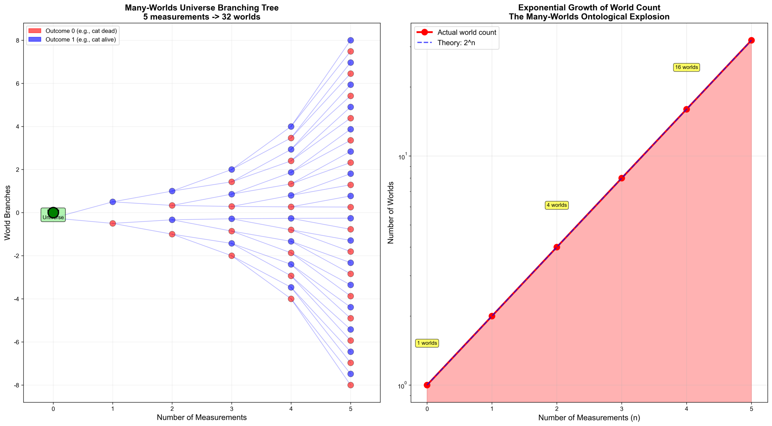
Next comes the core visualization: plotting the universe branching tree. The left panel uses a tree structure to show how worlds split in two after each measurement — red nodes represent “cat is dead” worlds, blue nodes represent “cat is alive” worlds. Notice how the number of nodes doubles at each level. This is the “ontological explosion” that the Many-Worlds Interpretation entails.
    def visualize_branching(self, n_measurements=5):
        """
        Visualize the universe branching tree
        """
        fig, (ax1, ax2) = plt.subplots(1, 2, figsize=(18, 10))

        # === Left panel: tree diagram ===
        self.initialize()

        # Track the number of worlds at each step
        steps = [0]
        world_counts = [1]

        # Calculate positions
        max_level = n_measurements
        level_positions = {}  # {level: [world_ids]}

        for level in range(max_level + 1):
            level_positions[level] = []

        # Initial world
        level_positions[0] = [0]

        # Draw the initial world
        ax1.scatter([0], [0], s=300, c='green', zorder=5,
                   edgecolors='black', linewidth=2)
        ax1.text(0, -0.3, 'Initial\nUniverse', ha='center', fontsize=9,
                bbox=dict(boxstyle='round', facecolor='lightgreen', alpha=0.7))

        # Perform measurements step by step
        for measurement in range(1, n_measurements + 1):
            n_worlds = self.quantum_measurement(n_outcomes=2)
            steps.append(measurement)
            world_counts.append(n_worlds)

            # Calculate positions for this level
            n_worlds_this_level = 2 ** measurement
            y_positions = np.linspace(-n_worlds_this_level/4,
                                     n_worlds_this_level/4,
                                     n_worlds_this_level)

            # Draw connecting lines and nodes
            prev_level_size = 2 ** (measurement - 1)
            prev_y_positions = np.linspace(-prev_level_size/4,
                                          prev_level_size/4,
                                          prev_level_size)

            for i in range(n_worlds_this_level):
                parent_idx = i // 2
                ax1.plot([measurement-1, measurement],
                        [prev_y_positions[parent_idx], y_positions[i]],
                        'b-', alpha=0.3, linewidth=1)
                color = 'red' if i % 2 == 0 else 'blue'
                ax1.scatter([measurement], [y_positions[i]],
                           s=100, c=color, zorder=5, alpha=0.6,
                           edgecolors='black', linewidth=0.5)

        ax1.set_xlabel('Number of Measurements', fontsize=13)
        ax1.set_ylabel('World Branches', fontsize=13)
        ax1.set_title(f'Many-Worlds Universe Branching Tree\n{n_measurements} measurements → {2**n_measurements} worlds',
                     fontsize=14, fontweight='bold')
        ax1.grid(True, alpha=0.2)
        ax1.set_xlim(-0.5, n_measurements + 0.5)

        red_patch = mpatches.Patch(color='red', label='Outcome 0 (e.g., cat dead)', alpha=0.6)
        blue_patch = mpatches.Patch(color='blue', label='Outcome 1 (e.g., cat alive)', alpha=0.6)
        ax1.legend(handles=[red_patch, blue_patch], fontsize=10)
The right panel uses a logarithmic scale to show the growth curve of the number of worlds. The key finding here: the growth is exponential. Just 100 quantum measurements would produce roughly 1.27 x 10^30 parallel worlds — and the universe experiences far more quantum events than that every single second.
        # === Right panel: world count growth ===
        ax2.plot(steps, world_counts, 'ro-', linewidth=3, markersize=10, label='Actual world count')
        ax2.fill_between(steps, 0, world_counts, alpha=0.3, color='red')

        theory_counts = [2**i for i in steps]
        ax2.plot(steps, theory_counts, 'b--', linewidth=2, label='Theory: 2^n', alpha=0.7)

        ax2.set_xlabel('Number of Measurements (n)', fontsize=13)
        ax2.set_ylabel('Number of Worlds', fontsize=13)
        ax2.set_title('Exponential Growth of World Count\nThe Many-Worlds Ontological Explosion',
                     fontsize=14, fontweight='bold')
        ax2.legend(fontsize=12)
        ax2.grid(True, alpha=0.3)
        ax2.set_yscale('log')

        for step, count in zip(steps[::2], world_counts[::2]):
            ax2.text(step, count * 1.5, f'{count} worlds',
                    ha='center', fontsize=9,
                    bbox=dict(boxstyle='round', facecolor='yellow', alpha=0.6))

        plt.tight_layout()
        plt.savefig('multiverse_branching.png', dpi=300, bbox_inches='tight')
        plt.show()

        # Data output
        print("\n" + "="*70)
        print("MANY-WORLDS UNIVERSE BRANCHING")
        print("="*70)
        print(f"\nInitial state: 1 universe")
        print(f"After 1 measurement: {2**1} worlds (universe splits in two)")
        print(f"After 2 measurements: {2**2} worlds")
        print(f"After 3 measurements: {2**3} worlds")
        print(f"After 4 measurements: {2**4} worlds")
        print(f"After 5 measurements: {2**5} worlds")
        print(f"\nAfter n measurements: 2^n worlds")
        print(f"\nExamples:")
        print(f"  * 10 measurements = {2**10:,} worlds")
        print(f"  * 20 measurements = {2**20:,} worlds")
        print(f"  * 30 measurements = {2**30:,} worlds")
        print(f"  * 100 measurements = {2**100:.2e} worlds")
        print(f"\nThe universe undergoes ~10^50 quantum events per second...")
        print(f"The number of worlds: beyond imagination!")
        print("="*70)
The second method, compare_interpretations, uses a four-panel figure to directly compare the worldviews of the Copenhagen interpretation, the Many-Worlds interpretation, and Huayan Buddhism. Copenhagen says “the wave function collapses — only one outcome occurs.” Many-Worlds says “the universe splits — all outcomes occur.” Huayan says “each dust mote contains infinite realms, all mutually interpenetrating.” Three frameworks, three fundamentally different understandings of what “reality” means.
    def compare_interpretations(self):
        """
        Compare different interpretations of quantum measurement
        """
        fig, axes = plt.subplots(2, 2, figsize=(16, 12))

        # === Copenhagen interpretation ===
        ax = axes[0, 0]
        ax.text(0.5, 0.7, 'Copenhagen Interpretation', ha='center', fontsize=16,
               fontweight='bold', transform=ax.transAxes)

        circle1 = plt.Circle((0.3, 0.5), 0.15, color='purple', alpha=0.5)
        ax.add_patch(circle1)
        ax.text(0.3, 0.5, 'Superposition\n|psi>', ha='center', va='center', fontsize=11)

        ax.annotate('', xy=(0.7, 0.6), xytext=(0.5, 0.5),
                   arrowprops=dict(arrowstyle='->', lw=3, color='red'))
        ax.text(0.6, 0.65, 'Measurement\nCollapse', ha='center', fontsize=10, color='red')

        circle2 = plt.Circle((0.7, 0.6), 0.1, color='red', alpha=0.7)
        ax.add_patch(circle2)
        ax.text(0.7, 0.6, '|0>', ha='center', va='center', fontsize=11,
               fontweight='bold', color='white')

        ax.text(0.7, 0.3, 'OR', ha='center', fontsize=12, fontweight='bold')

        circle3 = plt.Circle((0.7, 0.2), 0.1, color='blue', alpha=0.7)
        ax.add_patch(circle3)
        ax.text(0.7, 0.2, '|1>', ha='center', va='center', fontsize=11,
               fontweight='bold', color='white')

        ax.set_xlim(0, 1)
        ax.set_ylim(0, 1)
        ax.axis('off')

        ax.text(0.5, 0.05, 'Wave function collapses\nOnly one outcome', ha='center', fontsize=10,
               transform=ax.transAxes,
               bbox=dict(boxstyle='round', facecolor='lightcoral', alpha=0.7))

        # === Many-Worlds interpretation ===
        ax = axes[0, 1]
        ax.text(0.5, 0.7, 'Many-Worlds Interpretation', ha='center', fontsize=16,
               fontweight='bold', transform=ax.transAxes)

        circle1 = plt.Circle((0.3, 0.5), 0.15, color='purple', alpha=0.5)
        ax.add_patch(circle1)
        ax.text(0.3, 0.5, 'Superposition\n|psi>', ha='center', va='center', fontsize=11)

        ax.annotate('', xy=(0.7, 0.6), xytext=(0.5, 0.5),
                   arrowprops=dict(arrowstyle='->', lw=3, color='green'))
        ax.annotate('', xy=(0.7, 0.2), xytext=(0.5, 0.5),
                   arrowprops=dict(arrowstyle='->', lw=3, color='green'))
        ax.text(0.6, 0.4, 'Universe\nSplits', ha='center', fontsize=10, color='green')

        circle2 = plt.Circle((0.7, 0.6), 0.1, color='red', alpha=0.7)
        ax.add_patch(circle2)
        ax.text(0.7, 0.6, '|0>', ha='center', va='center', fontsize=11,
               fontweight='bold', color='white')
        ax.text(0.85, 0.6, 'World A', ha='left', fontsize=9)

        circle3 = plt.Circle((0.7, 0.2), 0.1, color='blue', alpha=0.7)
        ax.add_patch(circle3)
        ax.text(0.7, 0.2, '|1>', ha='center', va='center', fontsize=11,
               fontweight='bold', color='white')
        ax.text(0.85, 0.2, 'World B', ha='left', fontsize=9)

        ax.set_xlim(0, 1)
        ax.set_ylim(0, 1)
        ax.axis('off')

        ax.text(0.5, 0.05, 'Wave function never collapses\nAll outcomes occur', ha='center', fontsize=10,
               transform=ax.transAxes,
               bbox=dict(boxstyle='round', facecolor='lightgreen', alpha=0.7))
Finally, the Huayan worldview is represented with a central circle surrounded by twelve “realms,” illustrating the “one dust mote contains all directions” structure. The bottom-right summary panel lays out the core differences and commonalities of the three interpretations side by side, letting readers see at a glance that whether we look through the lens of quantum mechanics or Huayan Buddhism, both point toward the same conclusion: multiple realities coexist.
        # === Huayan Buddhism ===
        ax = axes[1, 0]
        ax.text(0.5, 0.9, 'Huayan: Infinite Interpenetration', ha='center', fontsize=16,
               fontweight='bold', transform=ax.transAxes)

        circle_center = plt.Circle((0.5, 0.5), 0.08, color='gold', alpha=0.8,
                                  edgecolor='black', linewidth=2)
        ax.add_patch(circle_center)
        ax.text(0.5, 0.5, 'One\nDust', ha='center', va='center', fontsize=10,
               fontweight='bold')

        n_worlds = 12
        angles = np.linspace(0, 2*np.pi, n_worlds, endpoint=False)
        for i, angle in enumerate(angles):
            x = 0.5 + 0.3 * np.cos(angle)
            y = 0.5 + 0.3 * np.sin(angle)
            circle = plt.Circle((x, y), 0.05, color='lightblue', alpha=0.6,
                               edgecolor='blue', linewidth=1)
            ax.add_patch(circle)
            ax.text(x, y, f'Realm\n{i+1}', ha='center', va='center', fontsize=7)
            ax.plot([0.5, x], [0.5, y], 'gray', alpha=0.3, linewidth=1)

        ax.set_xlim(0, 1)
        ax.set_ylim(0, 1)
        ax.set_aspect('equal')
        ax.axis('off')

        ax.text(0.5, 0.05, 'One dust mote contains infinite realms\nAll realms mutually contain each other', ha='center', fontsize=10,
               transform=ax.transAxes,
               bbox=dict(boxstyle='round', facecolor='lightyellow', alpha=0.7))

        # === Comparison summary ===
        ax = axes[1, 1]
        ax.axis('off')

        comparison_text = '''
        Copenhagen vs Many-Worlds vs Huayan

        Copenhagen Interpretation:
        * Wave function collapses
        * Only one outcome
        * Probability: fundamental uncertainty

        Many-Worlds Interpretation:
        * Wave function never collapses
        * All outcomes occur (different worlds)
        * Probability: which world "I" end up in

        Huayan Buddhism:
        * All phenomena coexist simultaneously
        * Infinite interpenetrating realms
        * Perception: determined by karma

        Common Ground:
        - Multiple "realities" coexist
        - Observer-relativity
        - Infinite possibilities
        '''

        ax.text(0.1, 0.5, comparison_text, fontsize=11, va='center',
               family='monospace',
               bbox=dict(boxstyle='round', facecolor='white', alpha=0.9,
                        edgecolor='black', linewidth=2))

        plt.tight_layout()
        plt.savefig('interpretations_comparison.png', dpi=300, bbox_inches='tight')
        plt.show()

# Run
simulator = MultiverseSimulator()
simulator.visualize_branching(n_measurements=5)
simulator.compare_interpretations()
Output:
– Figure 1: Universe branching tree (5 measurements → 32 worlds)
– Figure 2: Exponential growth of world count (log scale)
– Figure 3: Three-way interpretation comparison (Copenhagen, Many-Worlds, Huayan)
Staggering numbers:
10 measurements = 1,024 worlds
20 measurements = 1,048,576 worlds
100 measurements = 1.27 x 10^30 worlds
Model 2: How Many Worlds Do “You” Exist In?
This model brings the Many-Worlds Interpretation down to everyday life: if every life choice creates parallel worlds, how many versions of “you” exist simultaneously? We use a simple class to track how each decision multiplies the number of worlds.
class QuantumBiography:
    """
    Quantum Biography: How many worlds does "I" exist in?
    """

    def __init__(self):
        self.decisions = []

    def add_decision(self, description, n_choices=2):
        """
        Add a life decision
        description: description of the decision
        n_choices: number of possible choices
        """
        self.decisions.append({
            'description': description,
            'n_choices': n_choices
        })

    def calculate_parallel_lives(self):
        """
        Calculate the number of parallel lives
        """
        total_worlds = 1
        for decision in self.decisions:
            total_worlds *= decision['n_choices']
        return total_worlds
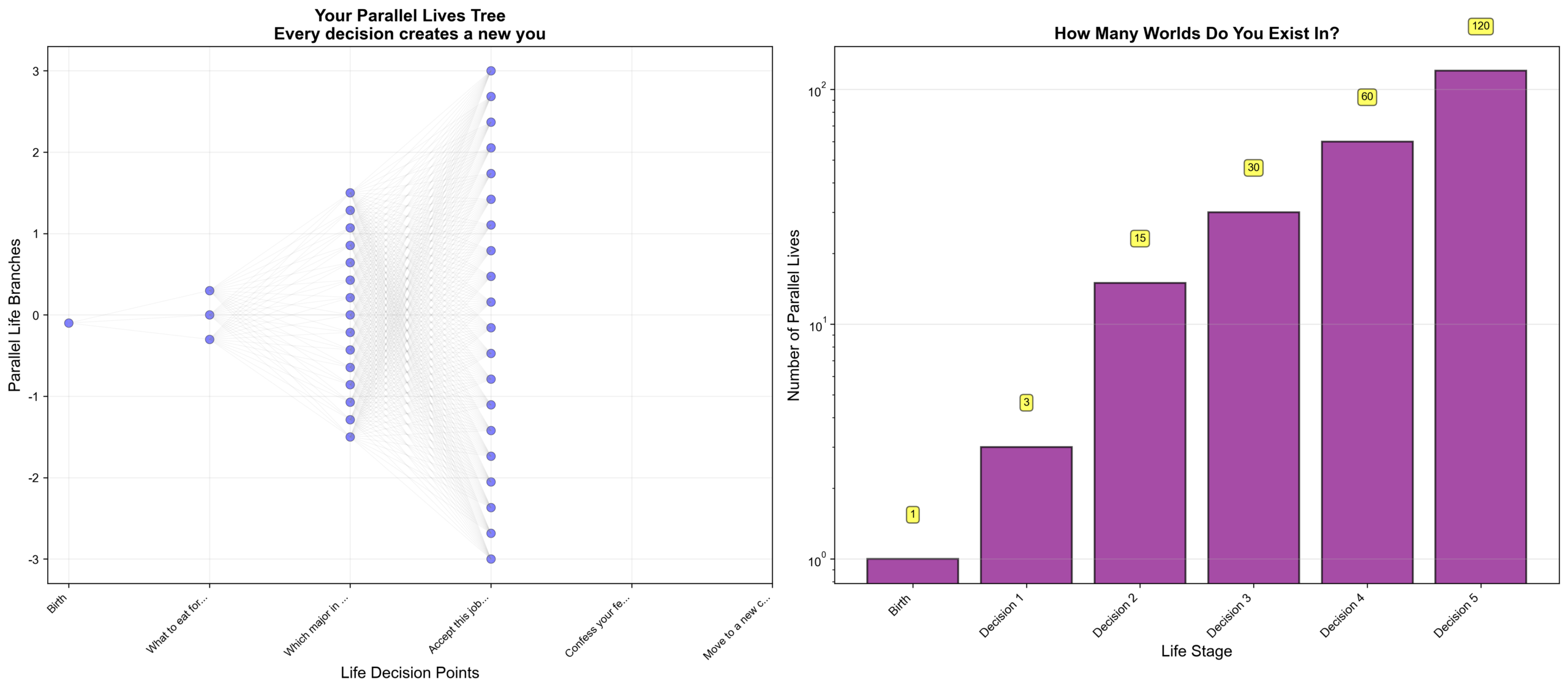
The left panel plots a life decision tree. We pick five typical life decisions — from “what to eat for breakfast” to “should I move to a new city.” Each node represents a version of “you” in a parallel world, with gray lines tracing the parent-child relationships between branches. The tree’s density increases rapidly with each level, visually capturing the “ontological explosion” effect.
    def visualize_life_tree(self):
        """
        Visualize the life decision tree
        """
        # Example decisions
        self.decisions = [
            {'description': 'What to eat for breakfast?', 'n_choices': 3},
            {'description': 'Which major in college?', 'n_choices': 5},
            {'description': 'Accept this job offer?', 'n_choices': 2},
            {'description': 'Confess your feelings?', 'n_choices': 2},
            {'description': 'Move to a new city?', 'n_choices': 2},
        ]

        fig, (ax1, ax2) = plt.subplots(1, 2, figsize=(18, 8))

        # === Left panel: decision tree ===
        cumulative_worlds = [1]
        for i, decision in enumerate(self.decisions):
            cumulative_worlds.append(cumulative_worlds[-1] * decision['n_choices'])

        for level, n_worlds in enumerate(cumulative_worlds):
            if level < 4:  # Only draw first few levels to avoid clutter
                y_positions = np.linspace(-n_worlds/10, n_worlds/10,
                                         min(n_worlds, 20))

                for y in y_positions[:min(n_worlds, 20)]:
                    ax1.scatter([level], [y], s=50, c='blue', alpha=0.5,
                              edgecolors='black', linewidth=0.5)

                if level > 0:
                    prev_n_worlds = cumulative_worlds[level-1]
                    prev_y_positions = np.linspace(-prev_n_worlds/10,
                                                   prev_n_worlds/10,
                                                   min(prev_n_worlds, 20))

                    for prev_y in prev_y_positions[:min(prev_n_worlds, 20)]:
                        for y in y_positions[:min(n_worlds, 20)]:
                            if abs(y - prev_y) < n_worlds/5:
                                ax1.plot([level-1, level], [prev_y, y],
                                       'gray', alpha=0.1, linewidth=0.5)

        ax1.set_xlabel('Life Decision Points', fontsize=13)
        ax1.set_ylabel('Parallel Life Branches', fontsize=13)
        ax1.set_title('Your Parallel Lives Tree\nEvery decision creates a new you',
                     fontsize=14, fontweight='bold')
        ax1.set_xticks(range(len(self.decisions) + 1))
        ax1.set_xticklabels(['Birth'] + [d['description'][:15]+'...'
                                       for d in self.decisions],
                           rotation=45, ha='right', fontsize=9)
        ax1.grid(True, alpha=0.2)
The right panel uses a bar chart to show the cumulative number of parallel lives. Five decisions (3 x 5 x 2 x 2 x 2) already produce 120 parallel versions of “you.” The data output poses an unsettling question: if you make 35,000 decisions per day, that is roughly 2^35000 worlds created in a single day. Huayan Buddhism’s response? All versions of “you” are real. “Self” was never singular to begin with.
        # === Right panel: parallel life count ===
        decision_labels = ['Birth'] + [f"Decision {i+1}" for i in range(len(self.decisions))]

        ax2.bar(range(len(cumulative_worlds)), cumulative_worlds,
               color='purple', alpha=0.7, edgecolor='black', linewidth=1.5)

        ax2.set_xlabel('Life Stage', fontsize=13)
        ax2.set_ylabel('Number of Parallel Lives', fontsize=13)
        ax2.set_title('How Many Worlds Do You Exist In?', fontsize=14, fontweight='bold')
        ax2.set_yscale('log')
        ax2.set_xticks(range(len(cumulative_worlds)))
        ax2.set_xticklabels(decision_labels, rotation=45, ha='right', fontsize=10)
        ax2.grid(True, alpha=0.3, axis='y')

        for i, n_worlds in enumerate(cumulative_worlds):
            ax2.text(i, n_worlds * 1.5, f'{n_worlds:,}',
                    ha='center', fontsize=9,
                    bbox=dict(boxstyle='round', facecolor='yellow', alpha=0.6))

        plt.tight_layout()
        plt.savefig('quantum_biography.png', dpi=300, bbox_inches='tight')
        plt.show()

        # Statistics
        total = self.calculate_parallel_lives()

        print("\n" + "="*70)
        print("YOUR PARALLEL LIVES")
        print("="*70)
        print("\nExample decisions:")
        for i, decision in enumerate(self.decisions, 1):
            print(f"  {i}. {decision['description']} ({decision['n_choices']} choices)")

        print(f"\nResult:")
        print(f"  * These decisions create {total:,} parallel versions of 'you'")
        print(f"  * Each version has a different life trajectory")
        print(f"  * Each version believes it is the only one")

        print(f"\nIn reality:")
        print(f"  * You make about 35,000 decisions per day")
        print(f"  * Each decision has on average 2-3 options")
        print(f"  * One day: ~2^35000 worlds")
        print(f"  * One lifetime: an incomprehensibly large number!")

        print(f"\nPhilosophical questions:")
        print(f"  * Which 'you' is the 'real you'?")
        print(f"  * Do the other versions of you wonder the same thing?")
        print(f"  * What does your 'uniqueness' even mean?")

        print(f"\nHuayan Buddhism's answer:")
        print(f"  * All versions of 'you' are real")
        print(f"  * 'Self' was never singular")
        print(f"  * 'One is all': each self contains every self")
        print("="*70)

# Run
biography = QuantumBiography()
biography.visualize_life_tree()
Output:
– Left panel: Life decision tree (branches multiply rapidly)
– Right panel: Parallel life count (log scale)
Mind-bending calculation:
5 decisions (3 x 5 x 2 x 2 x 2) = 120 parallel versions of “you”
35,000 decisions per day = 2^35000 ~ 10^10540 worlds!
The philosophical punch line:
Which “you” is the real you?
Answer: All of them.
Model 3: Huayan’s “One Dust Mote Contains All Directions” — Visualized
Huayan Buddhism says “within a single dust mote lie worlds as numerous as dust” — one particle contains infinite worlds. This “part contains whole” structure has a precise mathematical counterpart: fractals. We use four panels to illustrate this striking correspondence.
The first panel shows the classic Mandelbrot set. This set has a remarkable property: no matter which region you zoom into, you see structures similar to the whole. This is the mathematical equivalent of Huayan’s “subtle mutual containment” — every local region contains information about the entire structure.
def visualize_huayan_fractals():
    """
    Huayan's "One Dust Mote Contains All Directions" — Fractal visualization
    Demonstrates the structure of infinite recursion
    """

    fig = plt.figure(figsize=(18, 12))

    # === Panel 1: Mandelbrot set (the classic fractal example) ===
    ax1 = fig.add_subplot(2, 2, 1)

    def mandelbrot(c, max_iter=100):
        z = 0
        for n in range(max_iter):
            if abs(z) > 2:
                return n
            z = z*z + c
        return max_iter

    width, height = 800, 800
    xmin, xmax = -2.5, 1.0
    ymin, ymax = -1.25, 1.25

    x = np.linspace(xmin, xmax, width)
    y = np.linspace(ymin, ymax, height)
    X, Y = np.meshgrid(x, y)
    C = X + 1j*Y

    mandelbrot_set = np.zeros((height, width))
    for i in range(height):
        for j in range(width):
            mandelbrot_set[i, j] = mandelbrot(C[i, j], max_iter=50)

    im1 = ax1.imshow(mandelbrot_set, extent=[xmin, xmax, ymin, ymax],
                    cmap='hot', interpolation='bilinear', origin='lower')
    ax1.set_title('Mandelbrot Set: Infinite Detail\nZoom into any region and find similar structures',
                 fontsize=13, fontweight='bold')
    ax1.set_xlabel('Real Part')
    ax1.set_ylabel('Imaginary Part')
    plt.colorbar(im1, ax=ax1, label='Iteration Count')
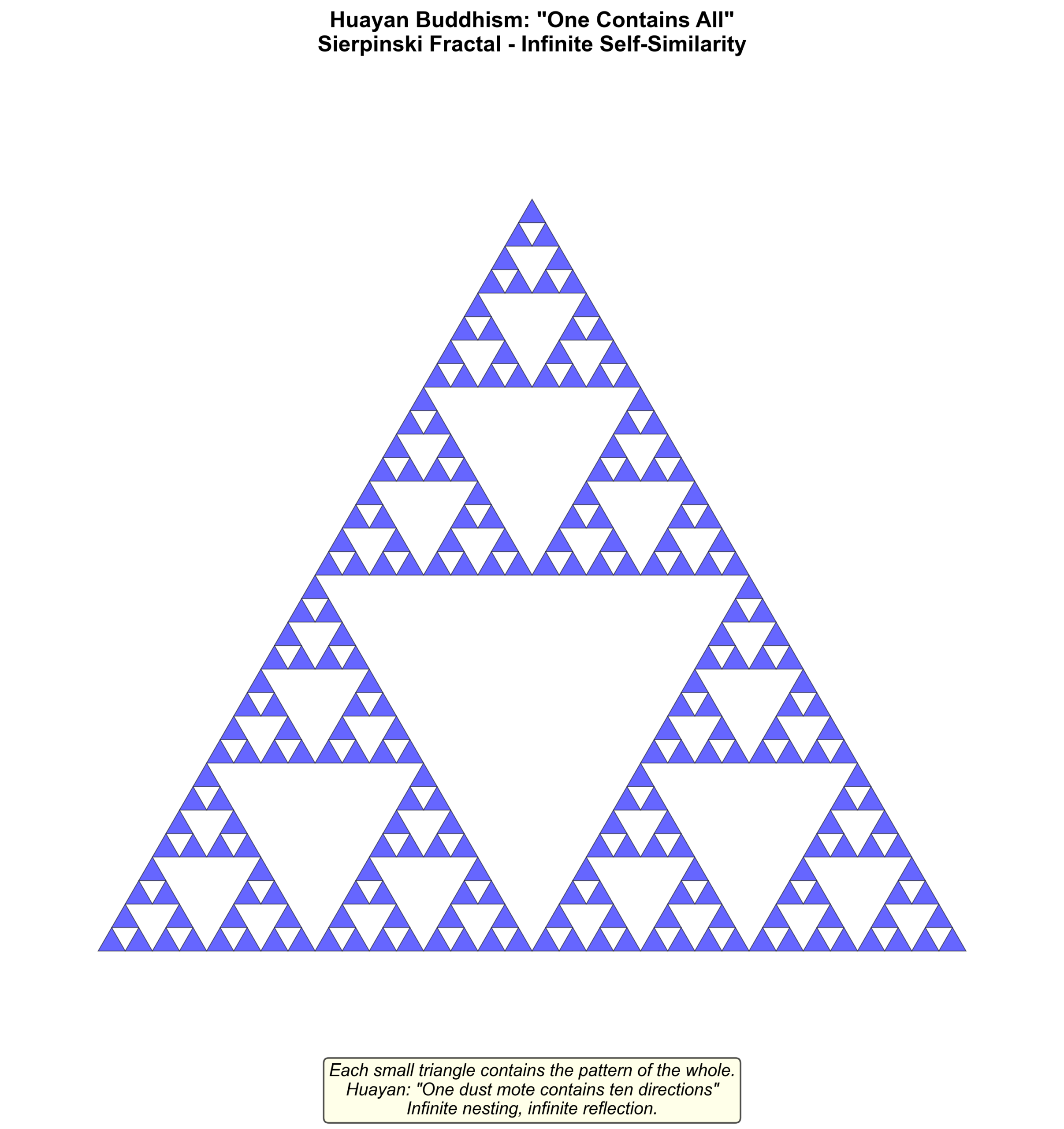
The second panel shows the Sierpinski triangle — another classic fractal. This structure is generated recursively: each triangle is subdivided into three smaller triangles, and each smaller triangle is a miniature copy of the whole. After five levels of recursion, the self-similarity between whole and part is unmistakable.
    # === Panel 2: Sierpinski triangle (recursive structure) ===
    ax2 = fig.add_subplot(2, 2, 2)

    def sierpinski(ax, order, points):
        """Draw a Sierpinski triangle"""
        if order == 0:
            triangle = plt.Polygon(points, fill=True,
                                  facecolor='blue', edgecolor='black',
                                  linewidth=0.5, alpha=0.6)
            ax.add_patch(triangle)
        else:
            p1, p2, p3 = points
            m12 = (p1 + p2) / 2
            m23 = (p2 + p3) / 2
            m31 = (p3 + p1) / 2
            sierpinski(ax, order-1, np.array([p1, m12, m31]))
            sierpinski(ax, order-1, np.array([m12, p2, m23]))
            sierpinski(ax, order-1, np.array([m31, m23, p3]))

    p1 = np.array([0, 0])
    p2 = np.array([1, 0])
    p3 = np.array([0.5, np.sqrt(3)/2])

    sierpinski(ax2, order=5, points=np.array([p1, p2, p3]))

    ax2.set_xlim(-0.1, 1.1)
    ax2.set_ylim(-0.1, 1.0)
    ax2.set_aspect('equal')
    ax2.axis('off')
    ax2.set_title('Sierpinski Triangle: Self-Similarity\nEach sub-triangle contains the whole structure',
                 fontsize=13, fontweight='bold')
The third panel directly visualizes Huayan’s world structure: a central “dust mote” is surrounded by six “realms,” each of which contains four smaller worlds. This is only two levels of recursion, but Huayan Buddhism speaks of “infinite interpenetration” — limitless recursion, with every level containing the complete whole.
    # === Panel 3: Huayan world structure ===
    ax3 = fig.add_subplot(2, 2, 3)

    circle_center = plt.Circle((0.5, 0.5), 0.1, color='gold', alpha=0.9,
                              edgecolor='black', linewidth=3)
    ax3.add_patch(circle_center)
    ax3.text(0.5, 0.5, 'One\nDust', ha='center', va='center', fontsize=14,
            fontweight='bold')

    n_layer1 = 6
    angles1 = np.linspace(0, 2*np.pi, n_layer1, endpoint=False)
    layer1_radius = 0.25

    for angle in angles1:
        x = 0.5 + layer1_radius * np.cos(angle)
        y = 0.5 + layer1_radius * np.sin(angle)

        circle = plt.Circle((x, y), 0.06, color='lightblue', alpha=0.7,
                           edgecolor='blue', linewidth=2)
        ax3.add_patch(circle)
        ax3.text(x, y, 'Realm', ha='center', va='center', fontsize=10)
        ax3.plot([0.5, x], [0.5, y], 'gray', alpha=0.5, linewidth=2)

        n_layer2 = 4
        angles2 = np.linspace(0, 2*np.pi, n_layer2, endpoint=False)
        layer2_radius = 0.03

        for angle2 in angles2:
            x2 = x + layer2_radius * np.cos(angle2)
            y2 = y + layer2_radius * np.sin(angle2)

            circle2 = plt.Circle((x2, y2), 0.015, color='lightgreen',
                                alpha=0.5, edgecolor='green', linewidth=0.5)
            ax3.add_patch(circle2)
            ax3.plot([x, x2], [y, y2], 'green', alpha=0.3, linewidth=0.5)

    ax3.set_xlim(0, 1)
    ax3.set_ylim(0, 1)
    ax3.set_aspect('equal')
    ax3.axis('off')
    ax3.set_title('Huayan: One Dust Mote Contains All Realms\nRealm within realm, without end',
                 fontsize=13, fontweight='bold')

    ax3.text(0.5, 0.05, '"Within one dust mote, worlds as numerous as dust"\nInfinite recursion',
            ha='center', fontsize=10, transform=ax3.transAxes,
            bbox=dict(boxstyle='round', facecolor='lightyellow', alpha=0.8))
The fourth panel is a summary comparison. The “self-similarity” of fractals, Huayan’s “subtle mutual containment,” and the Many-Worlds Interpretation’s “exponential branching” — all three point to the same deep insight: “infinity” is not about quantity being “very large.” It is a property of the structure itself.
    # === Panel 4: Comparison summary ===
    ax4 = fig.add_subplot(2, 2, 4)
    ax4.axis('off')

    text = '''
    Fractals vs Huayan "Infinite Interpenetration"

    Mathematical Fractals:
    * Self-similarity
    * Infinite detail
    * Part contains the whole
    * Zoom in to find the same structure

    Huayan "Infinite Interpenetration":
    * One dust mote contains all directions
    * All realms mutually contain each other
    * Subtle mutual containment
    * Infinite recursion

    Common Structure:
    - Infinite nesting
    - Part = Whole
    - Every level is complete
    - Without limit

    Many-Worlds Interpretation:
    * Universe constantly splits
    * Each world splits again
    * Branching tree grows without bound
    * Exponential explosion

    Shared Insight of All Three:
    "Infinity" is not "very large"
    It is a property of structure itself
    '''

    ax4.text(0.1, 0.5, text, fontsize=11, va='center',
            family='monospace',
            bbox=dict(boxstyle='round', facecolor='white', alpha=0.9,
                     edgecolor='black', linewidth=2))

    plt.tight_layout()
    plt.savefig('huayan_fractals.png', dpi=300, bbox_inches='tight')
    plt.show()

    print("\n" + "="*70)
    print("HUAYAN'S FRACTAL STRUCTURE")
    print("="*70)
    print("\nMathematical analogy:")
    print("  * Fractals: self-similar, infinite detail")
    print("  * Mandelbrot set: zoom into any region, find similar structures")
    print("  * Sierpinski triangle: each sub-triangle = the whole")
    print("\nDeep insight:")
    print("  'Infinity' is not a quantity concept")
    print("  It is a property of structure itself")
    print("  Part is whole, whole is part")
    print("="*70)

# Run
visualize_huayan_fractals()
Output:
– Panel 1: Mandelbrot set (infinite detail)
– Panel 2: Sierpinski triangle (self-similarity)
– Panel 3: Huayan world structure (one dust mote contains all)
– Panel 4: Comparison summary
Mathematical insight:
Fractal self-similarity = Huayan’s “subtle mutual containment”
Infinite nesting = infinite interpenetration
Part = Whole
Model 4: The Many-Worlds of Time — The Eighth Mysterious Gate
The Many-Worlds Interpretation doesn’t just transform our understanding of space — it radically overturns our notion of time. In the Many-Worlds framework, time is a tree that branches endlessly toward the future: the past is singular, but the future is multiple.
The left panel shows quantum temporal branching. Starting from a single initial world (t=0), each time step doubles the number of worlds. The size and opacity of nodes decrease with time, hinting that each world’s “weight” is gradually diluted through splitting. By t=4, sixteen parallel worlds coexist simultaneously.
def visualize_time_multiverse():
    """
    The Many-Worlds of Time
    Demonstrates how past, present, and future mutually contain one another
    """

    fig, (ax1, ax2) = plt.subplots(1, 2, figsize=(18, 9))

    # === Left panel: quantum temporal branching ===
    times = np.array([0, 1, 2, 3, 4])

    ax1.scatter([0], [0], s=500, c='green', zorder=5,
               edgecolors='black', linewidth=3)
    ax1.text(0, -0.5, 't=0\nInitial', ha='center', fontsize=10,
            bbox=dict(boxstyle='round', facecolor='lightgreen', alpha=0.7))

    # t=1: splits into 2
    y1 = [-1, 1]
    for y in y1:
        ax1.scatter([1], [y], s=300, c='blue', zorder=5,
                   edgecolors='black', linewidth=2, alpha=0.7)
        ax1.plot([0, 1], [0, y], 'b-', alpha=0.5, linewidth=2)

    # t=2: each splits into 2 more
    y2 = [-1.5, -0.5, 0.5, 1.5]
    for i, y in enumerate(y2):
        parent_y = y1[i//2]
        ax1.scatter([2], [y], s=200, c='red', zorder=5,
                   edgecolors='black', linewidth=1.5, alpha=0.6)
        ax1.plot([1, 2], [parent_y, y], 'r-', alpha=0.4, linewidth=1.5)

    # t=3: continue splitting
    y3 = np.linspace(-2, 2, 8)
    for i, y in enumerate(y3):
        parent_y = y2[i//2]
        ax1.scatter([3], [y], s=100, c='purple', zorder=5,
                   edgecolors='black', linewidth=1, alpha=0.5)
        ax1.plot([2, 3], [parent_y, y], 'purple', alpha=0.3, linewidth=1)

    # t=4: even more splitting
    y4 = np.linspace(-2.5, 2.5, 16)
    for i, y in enumerate(y4):
        parent_y = y3[i//2]
        ax1.scatter([4], [y], s=50, c='orange', zorder=5,
                   edgecolors='black', linewidth=0.5, alpha=0.4)
        ax1.plot([3, 4], [parent_y, y], 'orange', alpha=0.2, linewidth=0.5)

    ax1.set_xlabel('Time', fontsize=13)
    ax1.set_ylabel('World Branches', fontsize=13)
    ax1.set_title('Quantum Many-Worlds: Time Branches Toward the Future\nThe past is singular, the future is multiple',
                 fontsize=14, fontweight='bold')
    ax1.grid(True, alpha=0.2)
    ax1.set_xlim(-0.5, 4.5)
    ax1.set_ylim(-3, 3)

    ax1.text(2, 2.5, f't=2: {4} worlds', ha='center', fontsize=10,
            bbox=dict(boxstyle='round', facecolor='yellow', alpha=0.6))
    ax1.text(4, 2.8, f't=4: {16} worlds', ha='center', fontsize=10,
            bbox=dict(boxstyle='round', facecolor='yellow', alpha=0.6))
The right panel presents Huayan Buddhism’s radically different view of time. Three large circles represent past, present, and future, with bidirectional arrows showing that each contains the others. The eight smaller circles around them represent the first nine of Huayan’s “ten time-periods” (the tenth is all three times taken as one), showing how time in Huayan philosophy becomes a web of mutual interpenetration rather than a one-way arrow.
    # === Right panel: Huayan's ten time-periods ===
    past_center = np.array([0.2, 0.5])
    present_center = np.array([0.5, 0.5])
    future_center = np.array([0.8, 0.5])

    circle_past = plt.Circle(past_center, 0.15, color='blue', alpha=0.3,
                            edgecolor='blue', linewidth=3)
    ax2.add_patch(circle_past)
    ax2.text(past_center[0], past_center[1], 'Past',
            ha='center', va='center', fontsize=14, fontweight='bold')

    circle_present = plt.Circle(present_center, 0.15, color='green', alpha=0.3,
                               edgecolor='green', linewidth=3)
    ax2.add_patch(circle_present)
    ax2.text(present_center[0], present_center[1], 'Present',
            ha='center', va='center', fontsize=14, fontweight='bold')

    circle_future = plt.Circle(future_center, 0.15, color='red', alpha=0.3,
                              edgecolor='red', linewidth=3)
    ax2.add_patch(circle_future)
    ax2.text(future_center[0], future_center[1], 'Future',
            ha='center', va='center', fontsize=14, fontweight='bold')

    connections = [
        (past_center, present_center),
        (present_center, future_center),
        (past_center, future_center),
        (present_center, past_center),
        (future_center, present_center),
        (future_center, past_center),
    ]

    for start, end in connections:
        ax2.annotate('', xy=end, xytext=start,
                    arrowprops=dict(arrowstyle='->', lw=2, alpha=0.4,
                                  color='gray', connectionstyle="arc3,rad=.3"))

    positions_text = [
        (0.1, 0.8, 'Past of\nPast'),
        (0.1, 0.5, 'Present\nof Past'),
        (0.1, 0.2, 'Future\nof Past'),
        (0.5, 0.8, 'Past of\nPresent'),
        (0.5, 0.2, 'Future of\nPresent'),
        (0.9, 0.8, 'Past of\nFuture'),
        (0.9, 0.5, 'Present\nof Future'),
        (0.9, 0.2, 'Future\nof Future'),
    ]

    for x, y, label in positions_text:
        circle_small = plt.Circle((x, y), 0.06, color='yellow', alpha=0.5,
                                 edgecolor='orange', linewidth=1)
        ax2.add_patch(circle_small)
        ax2.text(x, y, label, ha='center', va='center', fontsize=7)

    ax2.set_xlim(0, 1)
    ax2.set_ylim(0, 1)
    ax2.set_aspect('equal')
    ax2.axis('off')
    ax2.set_title('Huayan "Ten Time-Periods": Times Mutually Contain Each Other\nPast holds future, future holds past',
                 fontsize=14, fontweight='bold')

    ax2.text(0.5, 0.05, '"The Eighth Gate: Distinct Dharmas of Ten Time-Periods"\nA single thought-moment contains all three times',
            ha='center', fontsize=10, transform=ax2.transAxes,
            bbox=dict(boxstyle='round', facecolor='lightyellow', alpha=0.8))

    plt.tight_layout()
    plt.savefig('time_multiverse.png', dpi=300, bbox_inches='tight')
    plt.show()
The data output summarizes the core difference between these two views of time. In quantum mechanics, time is unidirectional — from past to future, with branches only increasing. In Huayan Buddhism, time is bidirectionally interpenetrating — “a single thought-moment contains all three times,” and every instant encompasses all of time.
    print("\n" + "="*70)
    print("THE MANY-WORLDS OF TIME")
    print("="*70)

    print("\nQuantum Many-Worlds:")
    print("  * Time branches toward the future")
    print("  * The past: singular")
    print("  * The future: multiple (exponential growth)")
    print("  * Time is unidirectional")

    print("\nHuayan 'Ten Time-Periods':")
    print("  1. Past of the past")
    print("  2. Present of the past")
    print("  3. Future of the past")
    print("  4. Past of the present")
    print("  5. Present of the present")
    print("  6. Future of the present")
    print("  7. Past of the future")
    print("  8. Present of the future")
    print("  9. Future of the future")
    print("  10. All three times taken together as one")

    print("\nComparison:")
    print("  Quantum: time moves forward, branches increase")
    print("  Huayan: time has no fixed direction, all times mutually contain each other")
    print("="*70)

# Run
visualize_time_multiverse()
Output:
– Left panel: Quantum Many-Worlds (branching toward the future)
– Right panel: Huayan’s ten time-periods (mutual containment)
A revolution in how we think about time:
Quantum: the past is singular, the future is multiple
Huayan: past, present, and future mutually contain each other
“A single thought-moment contains all three times”
Why Is the Many-Worlds Interpretation Gaining Ground?
1. Mathematical Elegance
The Copenhagen interpretation requires:
– The Schrodinger equation (unitary evolution)
– + Wave function collapse (non-unitary)
– + The Born rule (probability)
The Many-Worlds interpretation requires only:
– The Schrodinger equation (unitary evolution)
That’s it. No additional postulates.
Occam’s Razor says: the simpler theory wins.
2. It Dissolves the “Measurement Problem”
Copenhagen’s difficulties:
– What counts as a “measurement”?
– When exactly does “collapse” happen?
– Why is measurement special?
Many-Worlds:
– There is no special process called “measurement”
– There are only interactions between quantum systems
– Decoherence naturally leads to branching
3. It Works for Quantum Cosmology
When studying the quantum state of the entire universe:
– There is no “external observer”
– Copenhagen doesn’t apply (who measures the universe?)
– Many-Worlds applies naturally
4. Compatibility with Quantum Computing
Quantum computing exploits superposition:
– Many-Worlds: computation occurs simultaneously across all worlds
– This picture helps in understanding quantum algorithms
5. Theorists Increasingly Prefer It
2022 survey of physicists:
– 42% support Many-Worlds
– Only 18% support Copenhagen
The trend is clear: Many-Worlds is becoming mainstream.
Did Huayan Buddhism “Foresee” Many-Worlds?
Not “Foresight” — Contemplative Insight
Huayan Buddhism did not arrive at its vision through experiments and equations.
It arrived there through contemplative observation of the mind — what Buddhists call direct insight into the nature of consciousness.
Two Paths to Knowledge
Western Physics:
1. Observe natural phenomena
2. Build mathematical models
3. Verify through experiment
4. Refine the theory
Path: outward investigation → mathematics → experiment
Huayan Buddhism:
1. Contemplate the nature of mind
2. Transcend conceptual thinking
3. Direct experiential insight
4. Express through language
Path: inward contemplation → insight → expression
Why Did They Reach Similar Conclusions?
Three possibilities:
1. Coincidence?
Unlikely. The structural parallels are too precise.
2. Did Western science borrow from Eastern thought?
Possible to some extent. But the Many-Worlds Interpretation is primarily grounded in mathematics.
3. Both traditions touched the same underlying reality?
The most compelling answer.
Different paths, converging truths:
– Physics: experiment → mathematics → theory
– Huayan: contemplation → insight → expression
Both discovered:
– “Reality” is not singular
– “Infinity” is a structural property
– “Parts” contain “wholes”
Deep Philosophical Questions
1. How many worlds do “I” exist in?
Many-Worlds answer:
Countless. Every quantum event splits “me.”
Huayan answer:
Countless. Every realm contains a version of “self.”
The Buddhist twist:
“Self” was never singular to begin with. The Buddhist concept of anatta (non-self) doesn’t mean “I don’t exist” — it means “I” has no fixed, independent essence. The idea that there is one unique, indivisible “me” was always an illusion.
2. Are the other versions of “me” really “me”?
Intuitive answer: No — they have different memories and experiences.
Deeper answer: Yes — they share a common origin and structure.
Huayan: “One is all.” Each “self” is every “self.”
3. Does free will still matter?
The worry: If all choices are realized somewhere, does any particular choice matter?
The response: Yes! Because your experience only happens in your world.
The other versions of “you” belong to their own worlds. They are not “you.”
4. What about moral responsibility?
The worry: If I commit a crime in one world but not in another, how do we assess moral responsibility?
The response: Each world has its own chain of cause and effect. You are responsible for your world.
5. What is “now”?
Many-Worlds: “Now” is a branching point. Countless versions of “now” exist simultaneously.
Huayan: “Now” contains both past and future. “A single thought-moment contains all three times.”
Questions for Reflection
-
If the Many-Worlds Interpretation says “all possibilities are realized,” what is the meaning of probability? Why do we observe specific probability distributions?
-
If countless versions of “me” exist, which one is the “real me”? Where does my uniqueness lie?
-
When Huayan Buddhism says “one dust mote contains all directions,” is this metaphor or literal truth?
-
Can time really “contain itself”? What does it mean to say “the past contains the future”?
-
If the Many-Worlds Interpretation is correct, would it change how you make decisions in life?
Next Episode Preview
Episode 7: Quantum Field Theory vs Buddhist Yogacara (“Mind-Only”) Philosophy
In 1949, Richard Feynman completed quantum electrodynamics (QED).
He discovered: Particles are not “things” — they are excitations of fields.
An electron is not a tiny ball.
It is an excitation mode of the electron field.
“Particles” are merely ripples in the field.
The Yogacara school of Buddhism (7th century) taught:
“The three realms are mind only; all phenomena are consciousness only.”
Everything we experience is a manifestation of consciousness.
There is no “external world” — only the transformations of consciousness.
In the next episode, we will explore:
– The complete framework of quantum field theory
– Feynman diagrams and virtual particles
– The vacuum is not empty: it seethes with quantum fluctuations
– Yogacara’s “eight consciousnesses” theory
– Simulating quantum fields with Python
The central question:
What is “matter”?
What is “mind”?
What is the relationship between them?