多世界與華嚴無盡：艾弗雷特遇見十法界

系列：量子力學遇見東方哲學 #06/12 | 閱讀時間：35-40分鐘 | Python (NumPy, Matplotlib)

作者：Wina @ Code & Cogito

被遺忘的天才

1957年，普林斯頓大學。

27歲的博士生休·艾弗雷特三世（Hugh Everett III）向導師約翰·惠勒（John Wheeler）提交了他的博士論文。

論文標題：《「相對狀態」的表述和量子力學》（“Relative State” Formulation of Quantum Mechanics）。

論文的核心觀點只有一句話：

波函數從不坍縮。

這意味著什麼？

意味著薛丁格的貓不是「打開盒子後，要麼死要麼活」。

而是：
– 打開盒子後，宇宙分裂成兩個世界
– 在世界A，貓死了
– 在世界B，貓活著
– 兩個世界都真實存在，但無法互相觀察

惠勒看完論文，驚呆了。

他說：「這…太瘋狂了。」

但他無法找到邏輯錯誤。

艾弗雷特堅持：「這是量子力學方程式的自然結果。沒有額外假設，沒有『坍縮』的神秘過程。波函數就按照薛丁格方程演化，僅此而已。」

1957年，論文發表在《現代物理評論》。

物理學界的反應：完全忽視。

波耳聽說後，憤怒地說：「這是胡說八道！」

艾弗雷特心灰意冷，離開物理學界，去了國防部工作。

1973年，物理學家布萊斯·德威特（Bryce DeWitt）重新發現了這個理論，給它起了一個更吸引人的名字：

「多世界詮釋」（Many-Worlds Interpretation, MWI）

1982年，艾弗雷特在睡夢中去世，享年51歲。

他的女兒伊莉莎白後來自殺，遺書中寫道：

「我要去平行宇宙找我的父親。」

今天，多世界詮釋是量子力學最流行的詮釋之一。

2022年的調查顯示：
– 18%的物理學家支持哥本哈根詮釋
– 42%的物理學家支持多世界詮釋

艾弗雷特的「瘋狂」想法，正在成為主流。

多世界詮釋：波函數從不坍縮

核心主張

多世界詮釋只有一個核心主張：

宇宙的波函數按照薛丁格方程演化，從不坍縮。

這個主張的後果是：

每次測量，宇宙分裂
不是「波函數坍縮到一個結果」
而是「宇宙分裂成多個分支，每個分支對應一個可能結果」
所有可能的結果都發生
薛丁格的貓：貓既死又活，在不同的世界
雙縫實驗：光子走了所有路徑，在不同的世界
「你」存在於無數個世界
每個世界有一個「你」
每個「你」有不同的經歷
但每個「你」都覺得自己是「唯一」的
世界之間不能通訊
分裂後的世界無法互相觀察
退相干（decoherence）使得分支迅速變得獨立
你永遠無法知道其他世界的「你」

數學表達

假設一個系統有兩個可能的狀態：|0⟩ 和 |1⟩。

初始態：|ψ⟩ = α|0⟩ + β|1⟩ （疊加態）

哥本哈根詮釋說：
– 測量後，波函數坍縮
– 機率 |α|² 得到 |0⟩
– 機率 |β|² 得到 |1⟩
– 坍縮是瞬間的、非么正的（違反薛丁格方程）

優點

多世界詮釋有幾個優點：

數學上更簡潔
只需要薛丁格方程
不需要額外的「坍縮」假設
波函數演化始終是么正的
解決了測量問題
哥本哈根：「測量」是什麼？何時發生坍縮？
多世界：沒有「測量」，只有相互作用和退相干
符合量子宇宙學
宇宙作為一個整體，沒有「外部觀察者」
波函數包含整個宇宙
多世界詮釋自然適用
可證偽性
原則上，如果能觀察到「世界合併」（退相干的逆過程）
就能證偽多世界詮釋
雖然在實踐中極其困難

缺點

多世界詮釋也有問題：

本體論爆炸
宇宙不斷分裂，產生無數個世界
每個世界都「真實」存在
這太「浪費」了？
機率的起源
如果所有結果都發生，為什麼有機率？
為什麼我們觀察到 |α|² 和 |β|²？
這是多世界詮釋的核心難題（「Born規則問題」）
無法驗證
我們永遠無法觀察其他世界
這是科學理論嗎？還是哲學猜測？
哲學上難以接受
「無數個我」存在？
「我」的獨特性在哪裡？
自由意志還有意義嗎？

華嚴宗的「重重無盡」：無限法界

公元7世紀，唐朝。

華嚴宗四祖澄觀（738-839）總結了華嚴宗的核心思想：

「法界緣起，重重無盡。」

《華嚴經》描述：

「一塵中有塵數剎，
一一剎有難思佛，
一一佛處眾會中，
我見恒演菩提行。」

翻譯：
– 一粒微塵中，包含無數世界（剎土）
– 每個世界中，有無數佛
– 每個佛都在講法
– 我見到無窮無盡的法界

這是什麼意思？

十世界、十佛剎

華嚴宗說：世界有「十重」：

此土世界 – 我們的娑婆世界
他方世界 – 其他無數世界
一佛剎 – 一個佛的世界
十佛剎 – 十方世界
百佛剎 – 百個世界
千佛剎 – 千個世界
萬佛剎 – 萬個世界
億佛剎 – 億個世界
不可說不可說佛剎 – 無數世界
微塵中佛剎 – 每個微塵都包含無數世界

關鍵：每個層次都包含下一層次的所有內容。

這形成了一個無限遞迴的結構。

「一即一切，一切即一」的極致

華嚴宗的核心思想是「一即一切，一切即一」。

在「重重無盡」中，這個思想達到極致：

一粒微塵 = 整個宇宙
不是比喻，是真實的包含
微塵中有無數世界
每個世界又有無數微塵
每個微塵又有無數世界
無限遞迴，無窮無盡

十玄門的第五門：微細相容安立門

華嚴宗十玄門的第五門叫「微細相容安立門」：

「於一微塵中，有大千經卷；
於一毛孔中，現無邊剎海。」

意思：
– 極小（微塵）可以包含極大（大千世界）
– 有限可以包含無限
– 一個點包含整個宇宙

這不是「縮小」，而是：
– 每個點都是完整的宇宙
– 宇宙不是「由點組成」
– 而是「每個點都是宇宙」

時間的重重無盡：十世隔法異成門

華嚴宗不僅說空間是重重無盡的，時間也是：

十玄門的第八門：「十世隔法異成門」

「十世」指：
1. 過去過去世
2. 過去現在世
3. 過去未來世
4. 現在過去世
5. 現在現在世
6. 現在未來世
7. 未來過去世
8. 未來現在世
9. 未來未來世
10. 三世各別總攝為一世

所有時間互相包含：
– 過去包含未來
– 未來包含過去
– 一念包含三世
– 時間是重重無盡的網絡

驚人的對應：多世界 vs 重重無盡

多世界詮釋	華嚴宗重重無盡
宇宙分裂	世界無盡
每次測量，宇宙分裂	一塵中有塵數剎
產生無數平行世界	剎剎相含，重重無盡
所有可能性都實現	一切法皆成
貓既死又活（不同世界）	萬法同時存在（不同剎土）
世界的層次	十佛剎
分支樹不斷增長	十重世界，層層包含
觀察者相對性	心識相對性
每個世界有一個「你」	每個剎土有一個「我」
你無法觀察其他世界的你	眾生無法見他方剎土
本體論爆炸	無盡法界
世界數量 = 2^n（n次測量）	不可說不可說佛剎
指數增長	無窮無盡

結構對應的深度

無限性（Infinity）
量子：測量次數 n → 世界數量 2^n → ∞
華嚴：一塵→塵數剎→剎中塵→剎剎中塵→∞
包含性（Containment）
量子：總波函數包含所有分支
華嚴：一塵包含一切剎，一切剎包含一塵
不可觀察性（Unobservability）
量子：退相干使得分支互不觀察
華嚴：眾生業力使得不見他方
全息性（Holography）
量子：每個分支包含整個宇宙的信息
華嚴：每個微塵包含整個法界

Python模型：看見無限的分裂

模型1：宇宙分裂模擬器

首先，我們建立多世界模擬器的核心類別。每個世界記錄自己的歷史路徑和振幅，每次量子測量都會讓所有現有世界分裂成新的分支。這個機制正是艾弗雷特理論的數學核心——波函數從不坍縮，只是不斷分裂。

import numpy as np
import matplotlib.pyplot as plt
from matplotlib.patches import Rectangle
import matplotlib.patches as mpatches

# 設定中文字體
plt.rcParams['font.sans-serif'] = ['Microsoft JhengHei', 'Arial']
plt.rcParams['axes.unicode_minus'] = False

class MultiverseSimulator:
    """
    多世界宇宙分裂模擬器
    展示：每次測量如何導致宇宙分裂
    """

    def __init__(self):
        self.worlds = []

    def initialize(self):
        """初始化：只有一個世界"""
        self.worlds = [{'id': 0, 'history': [], 'amplitude': 1.0}]

    def quantum_measurement(self, n_outcomes=2):
        """
        量子測量
        n_outcomes: 可能結果的數量（通常是2）
        """
        new_worlds = []

        for world in self.worlds:
            # 每個世界分裂成n_outcomes個新世界
            for outcome in range(n_outcomes):
                new_world = {
                    'id': len(new_worlds),
                    'history': world['history'] + [outcome],
                    'amplitude': world['amplitude'] / np.sqrt(n_outcomes)
                }
                new_worlds.append(new_world)

        self.worlds = new_worlds
        return len(self.worlds)

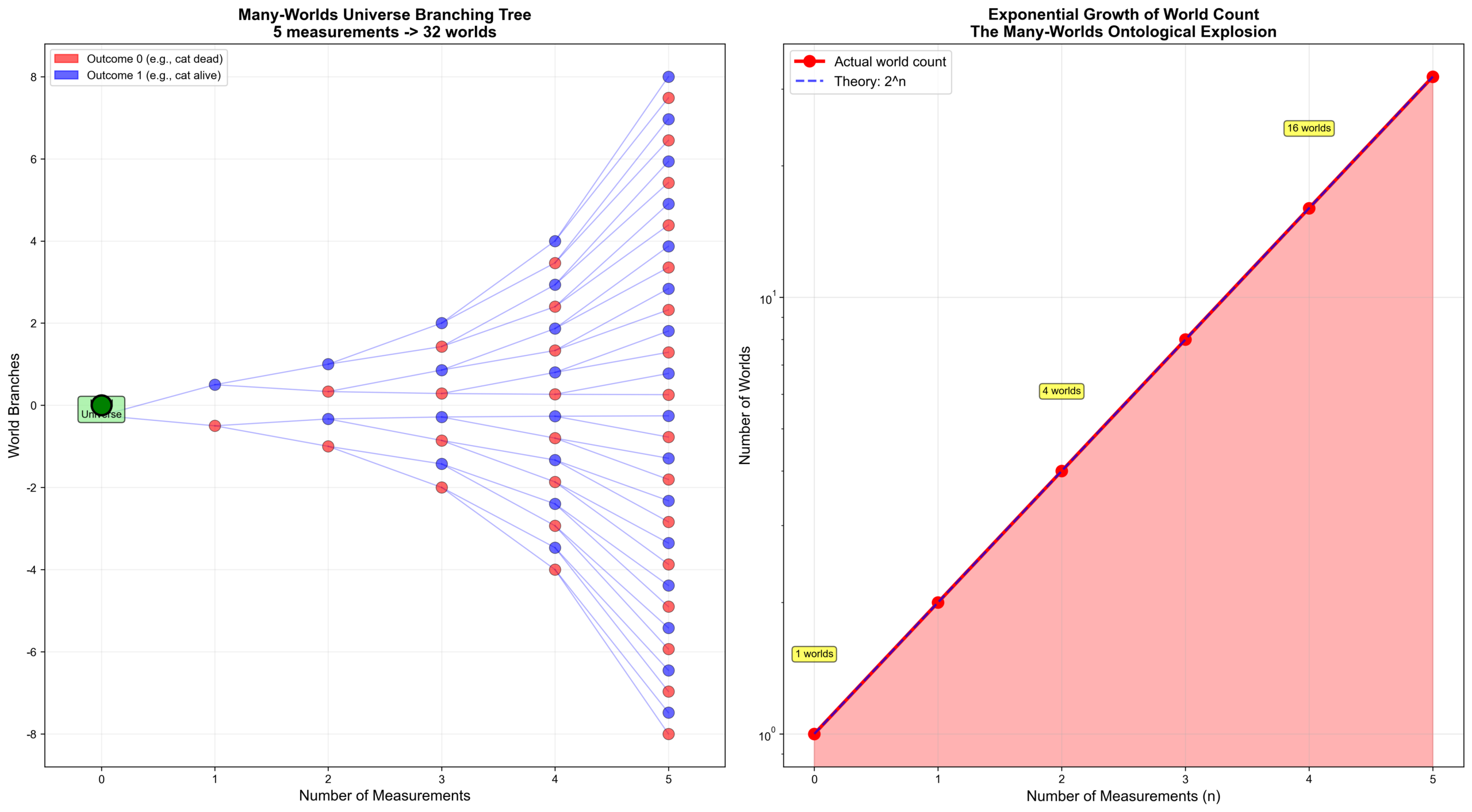
接下來是視覺化的核心：繪製宇宙分裂樹。左圖用樹狀結構展示每次測量後世界如何一分為二——紅色節點代表「貓死了」的世界，藍色代表「貓活著」的世界。注意每一層的節點數量如何倍增，這就是多世界詮釋所說的「本體論爆炸」。

    def visualize_branching(self, n_measurements=5):
        """
        視覺化宇宙分裂樹
        """
        fig, (ax1, ax2) = plt.subplots(1, 2, figsize=(18, 10))

        # === 左圖：樹狀圖 ===
        self.initialize()

        # 記錄每一步的世界數
        steps = [0]
        world_counts = [1]

        # 計算位置
        max_level = n_measurements
        level_positions = {}  # {level: [world_ids]}

        for level in range(max_level + 1):
            level_positions[level] = []

        # 初始世界
        level_positions[0] = [0]

        # 繪製初始世界
        ax1.scatter([0], [0], s=300, c='green', zorder=5,
                   edgecolors='black', linewidth=2)
        ax1.text(0, -0.3, '初始\n宇宙', ha='center', fontsize=9,
                bbox=dict(boxstyle='round', facecolor='lightgreen', alpha=0.7))

        # 逐步測量
        for measurement in range(1, n_measurements + 1):
            n_worlds = self.quantum_measurement(n_outcomes=2)
            steps.append(measurement)
            world_counts.append(n_worlds)

            # 計算這一層的位置
            n_worlds_this_level = 2 ** measurement
            y_positions = np.linspace(-n_worlds_this_level/4,
                                     n_worlds_this_level/4,
                                     n_worlds_this_level)

            # 繪製連接線和節點
            prev_level_size = 2 ** (measurement - 1)
            prev_y_positions = np.linspace(-prev_level_size/4,
                                          prev_level_size/4,
                                          prev_level_size)

            for i in range(n_worlds_this_level):
                parent_idx = i // 2
                ax1.plot([measurement-1, measurement],
                        [prev_y_positions[parent_idx], y_positions[i]],
                        'b-', alpha=0.3, linewidth=1)
                color = 'red' if i % 2 == 0 else 'blue'
                ax1.scatter([measurement], [y_positions[i]],
                           s=100, c=color, zorder=5, alpha=0.6,
                           edgecolors='black', linewidth=0.5)

        ax1.set_xlabel('測量次數', fontsize=13)
        ax1.set_ylabel('世界分支', fontsize=13)
        ax1.set_title(f'多世界宇宙分裂樹\n{n_measurements}次測量 → {2**n_measurements}個世界',
                     fontsize=14, fontweight='bold')
        ax1.grid(True, alpha=0.2)
        ax1.set_xlim(-0.5, n_measurements + 0.5)

        red_patch = mpatches.Patch(color='red', label='結果0（例如：貓死）', alpha=0.6)
        blue_patch = mpatches.Patch(color='blue', label='結果1（例如：貓活）', alpha=0.6)
        ax1.legend(handles=[red_patch, blue_patch], fontsize=10)

右圖用對數尺度展示世界數量的增長曲線。這裡的關鍵發現是：增長是指數級的。僅僅100次量子測量就會產生約 1.27 x 10^30 個平行世界——而宇宙每秒發生的量子事件遠不止此。

        # === 右圖：世界數量增長 ===
        ax2.plot(steps, world_counts, 'ro-', linewidth=3, markersize=10, label='實際世界數')
        ax2.fill_between(steps, 0, world_counts, alpha=0.3, color='red')

        theory_counts = [2**i for i in steps]
        ax2.plot(steps, theory_counts, 'b--', linewidth=2, label='理論：2^n', alpha=0.7)

        ax2.set_xlabel('測量次數 n', fontsize=13)
        ax2.set_ylabel('世界數量', fontsize=13)
        ax2.set_title('世界數量指數增長\n多世界本體論爆炸',
                     fontsize=14, fontweight='bold')
        ax2.legend(fontsize=12)
        ax2.grid(True, alpha=0.3)
        ax2.set_yscale('log')

        for step, count in zip(steps[::2], world_counts[::2]):
            ax2.text(step, count * 1.5, f'{count}個世界',
                    ha='center', fontsize=9,
                    bbox=dict(boxstyle='round', facecolor='yellow', alpha=0.6))

        plt.tight_layout()
        plt.savefig('multiverse_branching.png', dpi=300, bbox_inches='tight')
        plt.show()

        # 數據輸出
        print("\n" + "="*70)
        print("【多世界宇宙分裂】")
        print("="*70)
        print(f"\n初始：1個宇宙")
        print(f"測量1次：{2**1}個世界（宇宙分裂成2個）")
        print(f"測量2次：{2**2}個世界")
        print(f"測量3次：{2**3}個世界")
        print(f"測量4次：{2**4}個世界")
        print(f"測量5次：{2**5}個世界")
        print(f"\n測量n次：2^n 個世界")
        print(f"\n例子：")
        print(f"  * 測量10次 = {2**10:,}個世界")
        print(f"  * 測量20次 = {2**20:,}個世界")
        print(f"  * 測量30次 = {2**30:,}個世界")
        print(f"  * 測量100次 = {2**100:.2e}個世界")
        print(f"\n宇宙每秒發生約10^50次量子事件...")
        print(f"世界數量：無法想像的龐大！")
        print("="*70)

第二個方法 compare_interpretations 用四格圖直接對比哥本哈根詮釋、多世界詮釋與華嚴宗的世界觀。哥本哈根說「波函數坍縮，只有一個結果」；多世界說「宇宙分裂，所有結果都發生」；華嚴宗說「一塵含塵數剎，剎剎相含」。三種框架，三種對「實在」的不同理解。

    def compare_interpretations(self):
        """
        比較不同詮釋對測量的看法
        """
        fig, axes = plt.subplots(2, 2, figsize=(16, 12))

        # === 哥本哈根詮釋 ===
        ax = axes[0, 0]
        ax.text(0.5, 0.7, '哥本哈根詮釋', ha='center', fontsize=16,
               fontweight='bold', transform=ax.transAxes)

        circle1 = plt.Circle((0.3, 0.5), 0.15, color='purple', alpha=0.5)
        ax.add_patch(circle1)
        ax.text(0.3, 0.5, '疊加態\n|ψ⟩', ha='center', va='center', fontsize=11)

        ax.annotate('', xy=(0.7, 0.6), xytext=(0.5, 0.5),
                   arrowprops=dict(arrowstyle='->', lw=3, color='red'))
        ax.text(0.6, 0.65, '測量\n坍縮', ha='center', fontsize=10, color='red')

        circle2 = plt.Circle((0.7, 0.6), 0.1, color='red', alpha=0.7)
        ax.add_patch(circle2)
        ax.text(0.7, 0.6, '|0⟩', ha='center', va='center', fontsize=11,
               fontweight='bold', color='white')

        ax.text(0.7, 0.3, '或', ha='center', fontsize=12, fontweight='bold')

        circle3 = plt.Circle((0.7, 0.2), 0.1, color='blue', alpha=0.7)
        ax.add_patch(circle3)
        ax.text(0.7, 0.2, '|1⟩', ha='center', va='center', fontsize=11,
               fontweight='bold', color='white')

        ax.set_xlim(0, 1)
        ax.set_ylim(0, 1)
        ax.axis('off')

        ax.text(0.5, 0.05, '波函數坍縮\n只有一個結果', ha='center', fontsize=10,
               transform=ax.transAxes,
               bbox=dict(boxstyle='round', facecolor='lightcoral', alpha=0.7))

        # === 多世界詮釋 ===
        ax = axes[0, 1]
        ax.text(0.5, 0.7, '多世界詮釋', ha='center', fontsize=16,
               fontweight='bold', transform=ax.transAxes)

        circle1 = plt.Circle((0.3, 0.5), 0.15, color='purple', alpha=0.5)
        ax.add_patch(circle1)
        ax.text(0.3, 0.5, '疊加態\n|ψ⟩', ha='center', va='center', fontsize=11)

        ax.annotate('', xy=(0.7, 0.6), xytext=(0.5, 0.5),
                   arrowprops=dict(arrowstyle='->', lw=3, color='green'))
        ax.annotate('', xy=(0.7, 0.2), xytext=(0.5, 0.5),
                   arrowprops=dict(arrowstyle='->', lw=3, color='green'))
        ax.text(0.6, 0.4, '宇宙\n分裂', ha='center', fontsize=10, color='green')

        circle2 = plt.Circle((0.7, 0.6), 0.1, color='red', alpha=0.7)
        ax.add_patch(circle2)
        ax.text(0.7, 0.6, '|0⟩', ha='center', va='center', fontsize=11,
               fontweight='bold', color='white')
        ax.text(0.85, 0.6, '世界A', ha='left', fontsize=9)

        circle3 = plt.Circle((0.7, 0.2), 0.1, color='blue', alpha=0.7)
        ax.add_patch(circle3)
        ax.text(0.7, 0.2, '|1⟩', ha='center', va='center', fontsize=11,
               fontweight='bold', color='white')
        ax.text(0.85, 0.2, '世界B', ha='left', fontsize=9)

        ax.set_xlim(0, 1)
        ax.set_ylim(0, 1)
        ax.axis('off')

        ax.text(0.5, 0.05, '波函數不坍縮\n所有結果都發生', ha='center', fontsize=10,
               transform=ax.transAxes,
               bbox=dict(boxstyle='round', facecolor='lightgreen', alpha=0.7))

最後，華嚴宗的世界觀用中心圓與十二個圍繞的「剎土」來呈現「一塵含十方」的結構。右下角的總結框把三種詮釋的核心差異和共同點並列呈現，讓讀者一眼看出：無論是量子力學還是華嚴宗，都指向「多種實在並存」的結論。

        # === 華嚴宗 ===
        ax = axes[1, 0]
        ax.text(0.5, 0.9, '華嚴宗：重重無盡', ha='center', fontsize=16,
               fontweight='bold', transform=ax.transAxes)

        circle_center = plt.Circle((0.5, 0.5), 0.08, color='gold', alpha=0.8,
                                  edgecolor='black', linewidth=2)
        ax.add_patch(circle_center)
        ax.text(0.5, 0.5, '一塵', ha='center', va='center', fontsize=10,
               fontweight='bold')

        n_worlds = 12
        angles = np.linspace(0, 2*np.pi, n_worlds, endpoint=False)
        for i, angle in enumerate(angles):
            x = 0.5 + 0.3 * np.cos(angle)
            y = 0.5 + 0.3 * np.sin(angle)
            circle = plt.Circle((x, y), 0.05, color='lightblue', alpha=0.6,
                               edgecolor='blue', linewidth=1)
            ax.add_patch(circle)
            ax.text(x, y, f'剎{i+1}', ha='center', va='center', fontsize=7)
            ax.plot([0.5, x], [0.5, y], 'gray', alpha=0.3, linewidth=1)

        ax.set_xlim(0, 1)
        ax.set_ylim(0, 1)
        ax.set_aspect('equal')
        ax.axis('off')

        ax.text(0.5, 0.05, '一塵含塵數剎\n剎剎相含', ha='center', fontsize=10,
               transform=ax.transAxes,
               bbox=dict(boxstyle='round', facecolor='lightyellow', alpha=0.7))

        # === 對比總結 ===
        ax = axes[1, 1]
        ax.axis('off')

        comparison_text = '''
        【哥本哈根 vs 多世界 vs 華嚴】

        哥本哈根詮釋：
        * 波函數坍縮
        * 只有一個結果
        * 機率：本質不確定

        多世界詮釋：
        * 波函數不坍縮
        * 所有結果都發生（不同世界）
        * 機率：測量後「我」在哪個世界

        華嚴宗：
        * 一切法同時存在
        * 重重無盡的法界
        * 「我」見：依業力所見

        共同點：
        - 多種「實在」並存
        - 觀察者相對性
        - 無限的可能性
        '''

        ax.text(0.1, 0.5, comparison_text, fontsize=11, va='center',
               family='monospace',
               bbox=dict(boxstyle='round', facecolor='white', alpha=0.9,
                        edgecolor='black', linewidth=2))

        plt.tight_layout()
        plt.savefig('interpretations_comparison.png', dpi=300, bbox_inches='tight')
        plt.show()

# 執行
simulator = MultiverseSimulator()
simulator.visualize_branching(n_measurements=5)
simulator.compare_interpretations()

執行結果：
– 圖1：宇宙分裂樹（5次測量 → 32個世界）
– 圖2：世界數量指數增長（對數尺度）
– 圖3：三種詮釋對比（哥本哈根、多世界、華嚴）

震撼數據：

測量10次 = 1,024個世界
測量20次 = 1,048,576個世界
測量100次 = 1.27 x 10^30個世界

模型2：「我」在多少個世界裡？

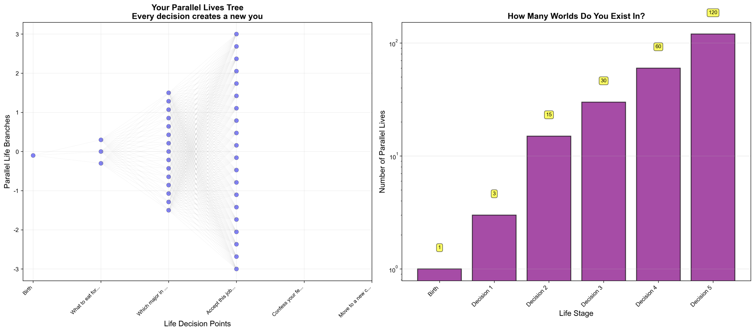
這個模型把多世界詮釋拉回日常生活：如果每個人生選擇都創造平行世界，那麼有多少個「你」同時存在？我們用一個簡單的類別來追蹤每個決定如何讓世界數量倍增。

class QuantumBiography:
    """
    量子自傳：「我」在多少個世界裡
    """

    def __init__(self):
        self.decisions = []

    def add_decision(self, description, n_choices=2):
        """
        添加一個人生決定
        description: 決定的描述
        n_choices: 選擇數量
        """
        self.decisions.append({
            'description': description,
            'n_choices': n_choices
        })

    def calculate_parallel_lives(self):
        """
        計算平行生命數量
        """
        total_worlds = 1
        for decision in self.decisions:
            total_worlds *= decision['n_choices']
        return total_worlds

左圖繪製人生決策樹。我們選了五個典型的人生決定——從「早餐吃什麼」到「搬到新城市嗎」。每個節點代表一個平行世界中的「你」，灰色連線追蹤各分支的父子關係。樹的密度隨層級迅速增加，視覺上呈現出「本體論爆炸」的效果。

    def visualize_life_tree(self):
        """
        視覺化人生決策樹
        """
        # 示例決策
        self.decisions = [
            {'description': '今天早餐吃什麼？', 'n_choices': 3},
            {'description': '大學選什麼專業？', 'n_choices': 5},
            {'description': '接受這份工作嗎？', 'n_choices': 2},
            {'description': '向TA告白嗎？', 'n_choices': 2},
            {'description': '搬到新城市嗎？', 'n_choices': 2},
        ]

        fig, (ax1, ax2) = plt.subplots(1, 2, figsize=(18, 8))

        # === 左圖：決策樹 ===
        cumulative_worlds = [1]
        for i, decision in enumerate(self.decisions):
            cumulative_worlds.append(cumulative_worlds[-1] * decision['n_choices'])

        for level, n_worlds in enumerate(cumulative_worlds):
            if level < 4:  # 只畫前幾層，避免太密
                y_positions = np.linspace(-n_worlds/10, n_worlds/10,
                                         min(n_worlds, 20))

                for y in y_positions[:min(n_worlds, 20)]:
                    ax1.scatter([level], [y], s=50, c='blue', alpha=0.5,
                              edgecolors='black', linewidth=0.5)

                if level > 0:
                    prev_n_worlds = cumulative_worlds[level-1]
                    prev_y_positions = np.linspace(-prev_n_worlds/10,
                                                   prev_n_worlds/10,
                                                   min(prev_n_worlds, 20))

                    for prev_y in prev_y_positions[:min(prev_n_worlds, 20)]:
                        for y in y_positions[:min(n_worlds, 20)]:
                            if abs(y - prev_y) < n_worlds/5:
                                ax1.plot([level-1, level], [prev_y, y],
                                       'gray', alpha=0.1, linewidth=0.5)

        ax1.set_xlabel('人生決策點', fontsize=13)
        ax1.set_ylabel('平行生命分支', fontsize=13)
        ax1.set_title('你的平行生命樹\n每個決定創造新的你',
                     fontsize=14, fontweight='bold')
        ax1.set_xticks(range(len(self.decisions) + 1))
        ax1.set_xticklabels(['出生'] + [d['description'][:8]+'...'
                                       for d in self.decisions],
                           rotation=45, ha='right', fontsize=9)
        ax1.grid(True, alpha=0.2)

右圖用柱狀圖直觀呈現平行生命的累積數量。五個決定（3 x 5 x 2 x 2 x 2）就已經產生120個平行的「你」。最後的數據輸出提出了一個令人不安的問題：如果你每天做35,000個決定，一天之內就會產生約 2^35000 個世界。華嚴宗的回答則是：所有的「你」都是真的，「我」本來就不是單一的。

        # === 右圖：平行生命數量 ===
        decision_labels = ['出生'] + [f"決定{i+1}" for i in range(len(self.decisions))]

        ax2.bar(range(len(cumulative_worlds)), cumulative_worlds,
               color='purple', alpha=0.7, edgecolor='black', linewidth=1.5)

        ax2.set_xlabel('人生階段', fontsize=13)
        ax2.set_ylabel('平行生命數量', fontsize=13)
        ax2.set_title('你存在於多少個世界？', fontsize=14, fontweight='bold')
        ax2.set_yscale('log')
        ax2.set_xticks(range(len(cumulative_worlds)))
        ax2.set_xticklabels(decision_labels, rotation=45, ha='right', fontsize=10)
        ax2.grid(True, alpha=0.3, axis='y')

        for i, n_worlds in enumerate(cumulative_worlds):
            ax2.text(i, n_worlds * 1.5, f'{n_worlds:,}',
                    ha='center', fontsize=9,
                    bbox=dict(boxstyle='round', facecolor='yellow', alpha=0.6))

        plt.tight_layout()
        plt.savefig('quantum_biography.png', dpi=300, bbox_inches='tight')
        plt.show()

        # 統計
        total = self.calculate_parallel_lives()

        print("\n" + "="*70)
        print("【你的平行生命】")
        print("="*70)
        print("\n示例決策：")
        for i, decision in enumerate(self.decisions, 1):
            print(f"  {i}. {decision['description']} ({decision['n_choices']}個選擇)")

        print(f"\n結果：")
        print(f"  * 這些決策創造了 {total:,} 個平行的「你」")
        print(f"  * 每個「你」有不同的人生軌跡")
        print(f"  * 每個「你」都覺得自己是「唯一」的")

        print(f"\n現實中：")
        print(f"  * 你每天做約 35,000 個決定")
        print(f"  * 每個決定平均有 2-3 個選擇")
        print(f"  * 一天：約 2^35000 個世界")
        print(f"  * 一生：無法計算的天文數字！")

        print(f"\n哲學問題：")
        print(f"  * 哪個「你」是「真正的你」？")
        print(f"  * 其他世界的「你」也這樣想嗎？")
        print(f"  * 「我」的獨特性在哪裡？")

        print(f"\n華嚴宗的答案：")
        print(f"  * 所有的「你」都是真的")
        print(f"  * 「我」本來就不是單一的")
        print(f"  * 「一即一切」：每個我包含一切我")
        print("="*70)

# 執行
biography = QuantumBiography()
biography.visualize_life_tree()

執行結果：
– 左圖：人生決策樹（分支不斷增加）
– 右圖：平行生命數量（對數尺度）

驚人計算：

5個決定（3 x 5 x 2 x 2 x 2）= 120個平行的「你」
每天35,000個決定 = 2^35000 ≈ 10^10540個世界！

哲學震撼：

哪個「你」是真正的你？
答案：所有的你都是真的。

模型3：華嚴宗的「一塵含十方」視覺化

華嚴宗說「一塵中有塵數剎」——一粒微塵包含無數世界。這種「部分包含整體」的結構，在數學上有一個精確的對應物：分形（fractal）。我們用四張圖來展示這個驚人的對應。

第一張圖是經典的 Mandelbrot 集。這個集合有一個神奇的特性：無論你放大到哪個區域，都會看到與整體相似的結構。這正是華嚴宗「微細相容」的數學版本——每個局部都包含整體的信息。

def visualize_huayan_fractals():
    """
    華嚴宗「一塵含十方」的分形視覺化
    展示：無限遞迴的結構
    """

    fig = plt.figure(figsize=(18, 12))

    # === 圖1：Mandelbrot集（分形的經典例子）===
    ax1 = fig.add_subplot(2, 2, 1)

    def mandelbrot(c, max_iter=100):
        z = 0
        for n in range(max_iter):
            if abs(z) > 2:
                return n
            z = z*z + c
        return max_iter

    width, height = 800, 800
    xmin, xmax = -2.5, 1.0
    ymin, ymax = -1.25, 1.25

    x = np.linspace(xmin, xmax, width)
    y = np.linspace(ymin, ymax, height)
    X, Y = np.meshgrid(x, y)
    C = X + 1j*Y

    mandelbrot_set = np.zeros((height, width))
    for i in range(height):
        for j in range(width):
            mandelbrot_set[i, j] = mandelbrot(C[i, j], max_iter=50)

    im1 = ax1.imshow(mandelbrot_set, extent=[xmin, xmax, ymin, ymax],
                    cmap='hot', interpolation='bilinear', origin='lower')
    ax1.set_title('Mandelbrot集：無限細節\n放大任何區域，都看到相似結構',
                 fontsize=13, fontweight='bold')
    ax1.set_xlabel('實部')
    ax1.set_ylabel('虛部')
    plt.colorbar(im1, ax=ax1, label='迭代次數')

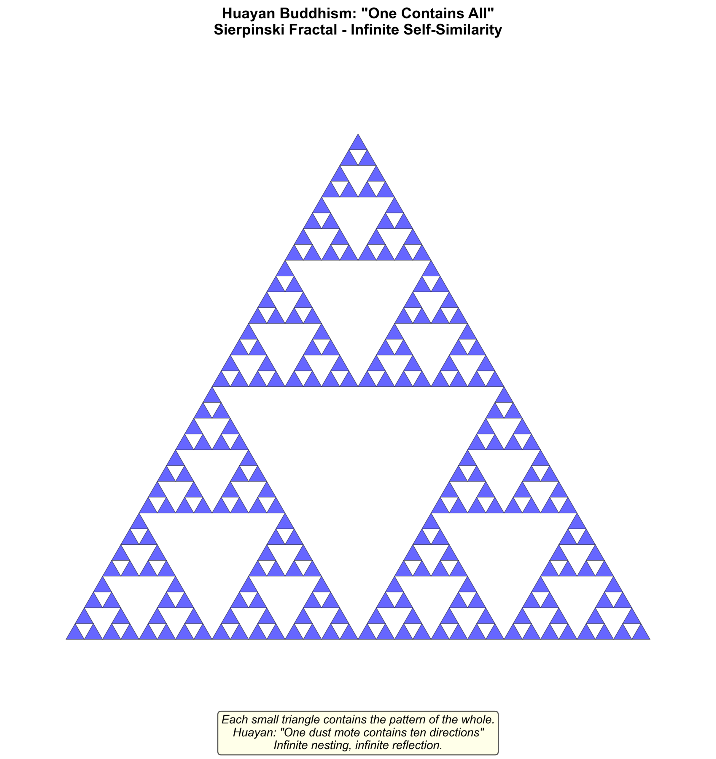
第二張圖是 Sierpinski 三角形——另一種經典分形。這個結構用遞迴方式生成：每個三角形再分成三個更小的三角形，每個小三角形又是整體的縮影。五層遞迴之後，整體與局部的自相似性一目瞭然。

    # === 圖2：Sierpinski三角形（遞迴結構）===
    ax2 = fig.add_subplot(2, 2, 2)

    def sierpinski(ax, order, points):
        """繪製Sierpinski三角形"""
        if order == 0:
            triangle = plt.Polygon(points, fill=True,
                                  facecolor='blue', edgecolor='black',
                                  linewidth=0.5, alpha=0.6)
            ax.add_patch(triangle)
        else:
            p1, p2, p3 = points
            m12 = (p1 + p2) / 2
            m23 = (p2 + p3) / 2
            m31 = (p3 + p1) / 2
            sierpinski(ax, order-1, np.array([p1, m12, m31]))
            sierpinski(ax, order-1, np.array([m12, p2, m23]))
            sierpinski(ax, order-1, np.array([m31, m23, p3]))

    p1 = np.array([0, 0])
    p2 = np.array([1, 0])
    p3 = np.array([0.5, np.sqrt(3)/2])

    sierpinski(ax2, order=5, points=np.array([p1, p2, p3]))

    ax2.set_xlim(-0.1, 1.1)
    ax2.set_ylim(-0.1, 1.0)
    ax2.set_aspect('equal')
    ax2.axis('off')
    ax2.set_title('Sierpinski三角形：自相似\n每個小三角形包含整體結構',
                 fontsize=13, fontweight='bold')

第三張圖直接視覺化華嚴宗的世界結構：中心是「一塵」，周圍環繞六個「剎土」，每個剎土又包含四個更小的世界。這只是兩層遞迴，但華嚴宗說的是「重重無盡」——無限層遞迴，每一層都完整包含整體。

    # === 圖3：華嚴宗結構圖 ===
    ax3 = fig.add_subplot(2, 2, 3)

    circle_center = plt.Circle((0.5, 0.5), 0.1, color='gold', alpha=0.9,
                              edgecolor='black', linewidth=3)
    ax3.add_patch(circle_center)
    ax3.text(0.5, 0.5, '一塵', ha='center', va='center', fontsize=14,
            fontweight='bold')

    n_layer1 = 6
    angles1 = np.linspace(0, 2*np.pi, n_layer1, endpoint=False)
    layer1_radius = 0.25

    for angle in angles1:
        x = 0.5 + layer1_radius * np.cos(angle)
        y = 0.5 + layer1_radius * np.sin(angle)

        circle = plt.Circle((x, y), 0.06, color='lightblue', alpha=0.7,
                           edgecolor='blue', linewidth=2)
        ax3.add_patch(circle)
        ax3.text(x, y, '剎', ha='center', va='center', fontsize=10)
        ax3.plot([0.5, x], [0.5, y], 'gray', alpha=0.5, linewidth=2)

        n_layer2 = 4
        angles2 = np.linspace(0, 2*np.pi, n_layer2, endpoint=False)
        layer2_radius = 0.03

        for angle2 in angles2:
            x2 = x + layer2_radius * np.cos(angle2)
            y2 = y + layer2_radius * np.sin(angle2)

            circle2 = plt.Circle((x2, y2), 0.015, color='lightgreen',
                                alpha=0.5, edgecolor='green', linewidth=0.5)
            ax3.add_patch(circle2)
            ax3.plot([x, x2], [y, y2], 'green', alpha=0.3, linewidth=0.5)

    ax3.set_xlim(0, 1)
    ax3.set_ylim(0, 1)
    ax3.set_aspect('equal')
    ax3.axis('off')
    ax3.set_title('華嚴宗：一塵含塵數剎\n剎剎相含，重重無盡',
                 fontsize=13, fontweight='bold')

    ax3.text(0.5, 0.05, '「一塵中有塵數剎，一一剎有難思佛」\n無限遞迴',
            ha='center', fontsize=10, transform=ax3.transAxes,
            bbox=dict(boxstyle='round', facecolor='lightyellow', alpha=0.8))

第四格是總結對照。分形的「自相似性」、華嚴宗的「微細相容」、多世界詮釋的「指數級分裂」——三者共同指向同一個深刻洞見：「無限」不是數量上的「很大」，而是結構本身的性質。

    # === 圖4：對應說明 ===
    ax4 = fig.add_subplot(2, 2, 4)
    ax4.axis('off')

    text = '''
    【分形 vs 華嚴「重重無盡」】

    數學分形：
    * 自相似性
    * 無限細節
    * 部分包含整體
    * 放大後看到相同結構

    華嚴宗「重重無盡」：
    * 一塵含十方
    * 剎剎相含
    * 微細相容
    * 無限遞迴

    共同結構：
    - 無限嵌套
    - 部分=整體
    - 每個層次都完整
    - 無窮無盡

    多世界詮釋：
    * 宇宙不斷分裂
    * 每個世界又分裂
    * 分支樹無限增長
    * 指數級爆炸

    三者的共同洞見：
    「無限」不是「很大」
    而是結構本身的性質
    '''

    ax4.text(0.1, 0.5, text, fontsize=11, va='center',
            family='monospace',
            bbox=dict(boxstyle='round', facecolor='white', alpha=0.9,
                     edgecolor='black', linewidth=2))

    plt.tight_layout()
    plt.savefig('huayan_fractals.png', dpi=300, bbox_inches='tight')
    plt.show()

    print("\n" + "="*70)
    print("【華嚴宗的分形結構】")
    print("="*70)
    print("\n數學類比：")
    print("  * 分形：自相似，無限細節")
    print("  * Mandelbrot集：放大任何區域都看到相似結構")
    print("  * Sierpinski三角形：每個小三角形=整體")
    print("\n深刻洞見：")
    print("  「無限」不是數量概念")
    print("  而是結構本身的性質")
    print("  部分即整體，整體即部分")
    print("="*70)

# 執行
visualize_huayan_fractals()

執行結果：
– 圖1：Mandelbrot集（無限細節）
– 圖2：Sierpinski三角形（自相似）
– 圖3：華嚴宗結構（一塵含十方）
– 圖4：對應說明

數學洞見：

分形的自相似性 = 華嚴宗的「微細相容」
無限嵌套 = 重重無盡
部分 = 整體

模型4：時間的多世界——十世隔法異成門

多世界詮釋不僅改變了我們對空間的理解，更徹底顛覆了時間觀。在多世界框架中，時間是一棵向未來不斷分裂的樹——過去唯一，未來多元。

左圖展示量子時間分支。從一個初始世界（t=0）出發，每個時間步都讓世界數倍增。節點的大小和透明度隨時間遞減，暗示每個世界的「權重」在分裂中逐漸稀釋。到 t=4 時，已經有16個平行世界同時存在。

def visualize_time_multiverse():
    """
    時間的多世界
    展示：過去、現在、未來如何互相包含
    """

    fig, (ax1, ax2) = plt.subplots(1, 2, figsize=(18, 9))

    # === 左圖：量子力學的時間分支 ===
    times = np.array([0, 1, 2, 3, 4])

    ax1.scatter([0], [0], s=500, c='green', zorder=5,
               edgecolors='black', linewidth=3)
    ax1.text(0, -0.5, 't=0\n初始', ha='center', fontsize=10,
            bbox=dict(boxstyle='round', facecolor='lightgreen', alpha=0.7))

    # t=1: 分裂成2個
    y1 = [-1, 1]
    for y in y1:
        ax1.scatter([1], [y], s=300, c='blue', zorder=5,
                   edgecolors='black', linewidth=2, alpha=0.7)
        ax1.plot([0, 1], [0, y], 'b-', alpha=0.5, linewidth=2)

    # t=2: 每個再分裂成2個
    y2 = [-1.5, -0.5, 0.5, 1.5]
    for i, y in enumerate(y2):
        parent_y = y1[i//2]
        ax1.scatter([2], [y], s=200, c='red', zorder=5,
                   edgecolors='black', linewidth=1.5, alpha=0.6)
        ax1.plot([1, 2], [parent_y, y], 'r-', alpha=0.4, linewidth=1.5)

    # t=3: 繼續分裂
    y3 = np.linspace(-2, 2, 8)
    for i, y in enumerate(y3):
        parent_y = y2[i//2]
        ax1.scatter([3], [y], s=100, c='purple', zorder=5,
                   edgecolors='black', linewidth=1, alpha=0.5)
        ax1.plot([2, 3], [parent_y, y], 'purple', alpha=0.3, linewidth=1)

    # t=4: 更多分裂
    y4 = np.linspace(-2.5, 2.5, 16)
    for i, y in enumerate(y4):
        parent_y = y3[i//2]
        ax1.scatter([4], [y], s=50, c='orange', zorder=5,
                   edgecolors='black', linewidth=0.5, alpha=0.4)
        ax1.plot([3, 4], [parent_y, y], 'orange', alpha=0.2, linewidth=0.5)

    ax1.set_xlabel('時間', fontsize=13)
    ax1.set_ylabel('世界分支', fontsize=13)
    ax1.set_title('量子多世界：時間向未來分裂\n過去唯一，未來多元',
                 fontsize=14, fontweight='bold')
    ax1.grid(True, alpha=0.2)
    ax1.set_xlim(-0.5, 4.5)
    ax1.set_ylim(-3, 3)

    ax1.text(2, 2.5, f't=2: {4}個世界', ha='center', fontsize=10,
            bbox=dict(boxstyle='round', facecolor='yellow', alpha=0.6))
    ax1.text(4, 2.8, f't=4: {16}個世界', ha='center', fontsize=10,
            bbox=dict(boxstyle='round', facecolor='yellow', alpha=0.6))

右圖呈現華嚴宗截然不同的時間觀。三個大圓代表過去、現在、未來，雙向箭頭表示它們彼此包含。周圍的八個小圓是華嚴宗「十世」的前九世（第十世是三世總攝為一），展示了時間如何在華嚴哲學中成為一張互相穿透的網絡，而非單向的箭頭。

    # === 右圖：華嚴宗的十世 ===
    past_center = np.array([0.2, 0.5])
    present_center = np.array([0.5, 0.5])
    future_center = np.array([0.8, 0.5])

    circle_past = plt.Circle(past_center, 0.15, color='blue', alpha=0.3,
                            edgecolor='blue', linewidth=3)
    ax2.add_patch(circle_past)
    ax2.text(past_center[0], past_center[1], '過去',
            ha='center', va='center', fontsize=14, fontweight='bold')

    circle_present = plt.Circle(present_center, 0.15, color='green', alpha=0.3,
                               edgecolor='green', linewidth=3)
    ax2.add_patch(circle_present)
    ax2.text(present_center[0], present_center[1], '現在',
            ha='center', va='center', fontsize=14, fontweight='bold')

    circle_future = plt.Circle(future_center, 0.15, color='red', alpha=0.3,
                              edgecolor='red', linewidth=3)
    ax2.add_patch(circle_future)
    ax2.text(future_center[0], future_center[1], '未來',
            ha='center', va='center', fontsize=14, fontweight='bold')

    connections = [
        (past_center, present_center),
        (present_center, future_center),
        (past_center, future_center),
        (present_center, past_center),
        (future_center, present_center),
        (future_center, past_center),
    ]

    for start, end in connections:
        ax2.annotate('', xy=end, xytext=start,
                    arrowprops=dict(arrowstyle='->', lw=2, alpha=0.4,
                                  color='gray', connectionstyle="arc3,rad=.3"))

    positions_text = [
        (0.1, 0.8, '過去\n過去'),
        (0.1, 0.5, '過去\n現在'),
        (0.1, 0.2, '過去\n未來'),
        (0.5, 0.8, '現在\n過去'),
        (0.5, 0.2, '現在\n未來'),
        (0.9, 0.8, '未來\n過去'),
        (0.9, 0.5, '未來\n現在'),
        (0.9, 0.2, '未來\n未來'),
    ]

    for x, y, label in positions_text:
        circle_small = plt.Circle((x, y), 0.06, color='yellow', alpha=0.5,
                                 edgecolor='orange', linewidth=1)
        ax2.add_patch(circle_small)
        ax2.text(x, y, label, ha='center', va='center', fontsize=7)

    ax2.set_xlim(0, 1)
    ax2.set_ylim(0, 1)
    ax2.set_aspect('equal')
    ax2.axis('off')
    ax2.set_title('華嚴宗「十世」：時間互相包含\n過去含未來，未來含過去',
                 fontsize=14, fontweight='bold')

    ax2.text(0.5, 0.05, '「十世隔法異成門」\n一念含三世，三世互攝',
            ha='center', fontsize=10, transform=ax2.transAxes,
            bbox=dict(boxstyle='round', facecolor='lightyellow', alpha=0.8))

    plt.tight_layout()
    plt.savefig('time_multiverse.png', dpi=300, bbox_inches='tight')
    plt.show()

數據輸出總結了兩種時間觀的核心差異。量子力學的時間是單向的——從過去到未來，分支只增不減。華嚴宗的時間是雙向互攝的——「一念含三世」，每個瞬間都包含所有時間。

    print("\n" + "="*70)
    print("【時間的多世界】")
    print("="*70)

    print("\n量子力學多世界：")
    print("  * 時間向未來分裂")
    print("  * 過去：唯一")
    print("  * 未來：多元（指數增長）")
    print("  * 時間是單向的")

    print("\n華嚴宗「十世」：")
    print("  1. 過去過去世")
    print("  2. 過去現在世")
    print("  3. 過去未來世")
    print("  4. 現在過去世")
    print("  5. 現在現在世")
    print("  6. 現在未來世")
    print("  7. 未來過去世")
    print("  8. 未來現在世")
    print("  9. 未來未來世")
    print("  10. 三世各別總攝為一世")

    print("\n對比：")
    print("  量子：時間向前，分支增加")
    print("  華嚴：時間無向，互相包含")
    print("="*70)

# 執行
visualize_time_multiverse()

執行結果：
– 左圖：量子多世界（向未來分裂）
– 右圖：華嚴宗十世（互相包含）

時間觀革命：

量子：過去唯一，未來多元
華嚴：過去、現在、未來互相包含
「一念含三世」

為什麼多世界詮釋越來越被接受？

1. 數學上更簡潔

哥本哈根詮釋需要：
– 薛丁格方程（么正演化）
– + 波函數坍縮（非么正）
– + Born規則（機率）

多世界詮釋只需要：
– 薛丁格方程（么正演化）

就這樣。沒有額外假設。

奧卡姆剃刀原則：理論越簡單越好。

2. 解決了「測量問題」

哥本哈根詮釋的困難：
– 什麼算「測量」？
– 何時發生「坍縮」？
– 為什麼測量特殊？

多世界詮釋：
– 沒有「測量」這個特殊過程
– 只有量子系統之間的相互作用
– 退相干自然導致分支

3. 適用於量子宇宙學

研究整個宇宙的量子態時：
– 沒有「外部觀察者」
– 哥本哈根詮釋不適用（誰來測量宇宙？）
– 多世界詮釋自然適用

4. 與量子計算的相容性

量子計算利用疊加態：
– 多世界詮釋：計算在所有世界同時進行
– 這個圖像幫助理解量子算法

5. 理論物理學家的偏好

2022年調查：
– 42% 支持多世界詮釋
– 只有 18% 支持哥本哈根詮釋

趨勢：多世界正在成為主流。

華嚴宗如何「預見」了多世界？

不是「預見」，是「體悟」

華嚴宗不是通過實驗和數學「發現」多世界。

而是通過觀照心識「體悟」無盡法界。

兩種認識路徑

西方物理學：
1. 觀察自然現象
2. 建立數學模型
3. 實驗驗證
4. 修正理論

路徑：外求 → 數學 → 實驗

華嚴宗：
1. 觀照心識
2. 超越概念
3. 直接體悟
4. 言說表達

路徑：內觀 → 體悟 → 言說

為什麼抵達相似結論？

三種可能：

1. 巧合？

不太可能。結構對應太精確。

2. 西方科學受東方影響？

有一定可能。但多世界詮釋主要基於數學。

3. 兩者都觸及了實在的本質？

最可能的答案。

不同的路徑，相同的真理：
– 物理學：實驗 → 數學 → 理論
– 華嚴宗：觀照 → 體悟 → 言說

兩者都發現：
– 「實在」不是單一的
– 「無限」是結構的性質
– 「部分」包含「整體」

深刻的哲學問題

1. 「我」在多少個世界裡？

多世界答案：
無數個。每次量子事件，「我」都分裂。

華嚴答案：
無數個。每個剎土有一個「我」。

佛教答案：
「我」本來就不是單一的。「無我」不是沒有我，是「我」無固定自性。

2. 其他世界的「我」是「我」嗎？

直覺： 不是，因為有不同的記憶和經歷。

深層： 是，因為有共同的起源和結構。

華嚴： 「一即一切」。每個「我」都是所有「我」。

3. 自由意志還有意義嗎？

擔心： 如果所有選擇都發生，我的選擇還重要嗎？

回答： 重要！因為「你」的經歷只在「你的」世界發生。

其他世界的「你」是其他世界的「你」，不是「你」。

4. 道德責任呢？

擔心： 如果我在某個世界殺人，在另一個世界沒殺，道德如何判斷？

回答： 每個世界有自己的因果。你對「你的」世界負責。

5. 「現在」是什麼？

多世界： 「現在」是分支點。無數個「現在」同時存在。

華嚴： 「現在」包含過去和未來。「一念含三世」。

思考題

多世界詮釋說「所有可能都發生」，那麼機率的意義是什麼？為什麼我們觀察到特定的機率分佈？
如果無數個「我」存在，哪個「我」是「真正的我」？「我」的獨特性在哪裡？
華嚴宗說「一塵含十方」，這是比喻還是字面真理？
時間真的可以「互相包含」嗎？「過去包含未來」是什麼意思？
如果多世界詮釋是對的，這會改變你的人生選擇嗎？

下集預告

第7集：量子場論 vs 佛教的「唯識」

1949年，理查德·費曼（Richard Feynman）完成了量子電動力學（QED）。

他發現：粒子不是「東西」，而是「場的激發」。

電子不是一個「小球」。
而是電子場的一個激發模式。
「粒子」只是場的漣漪。

唯識宗（7世紀）說：

「三界唯心，萬法唯識。」
一切法都是心識的顯現。
沒有「外境」，只有「識」的變現。

下一集，我們將探索：
– 量子場論的完整理論
– 費曼圖與虛粒子
– 真空不空：充滿量子漲落
– 唯識宗的「八識」理論
– 用Python模擬量子場

核心問題：

「物質」是什麼？
「心」是什麼？
物質和心的關係是什麼？