The Uncertainty Principle vs Buddhist “Emptiness” — Nothing Has an Inherent Nature
Series: Quantum Mechanics Meets Eastern Philosophy #04/12 | Reading time: 30-35 min | Python (NumPy, Matplotlib, SciPy, NetworkX)
Author: Wina @ Code & Cogito
A Sleepless Night on Helgoland
February 1927. The island of Helgoland, off the coast of Germany in the North Sea.
Twenty-three-year-old Werner Heisenberg stood alone at the edge of a cliff, staring out at the dark ocean.
He had come to this remote island to escape his hay fever in Munich. But here, he would complete one of the most profound discoveries in the history of physics.
The night before, he had finally worked out the complete formulation of matrix mechanics. At 3 a.m., he calculated the energy levels of the hydrogen atom — and they matched experiment perfectly.
Too excited to sleep, he climbed a rocky outcrop on the island and waited for sunrise.
As the sun rose, a realization struck him:
A particle does not have a simultaneously well-defined position and momentum.
Not “it has them but we can’t measure them accurately” — rather, “they genuinely do not exist at the same time.”
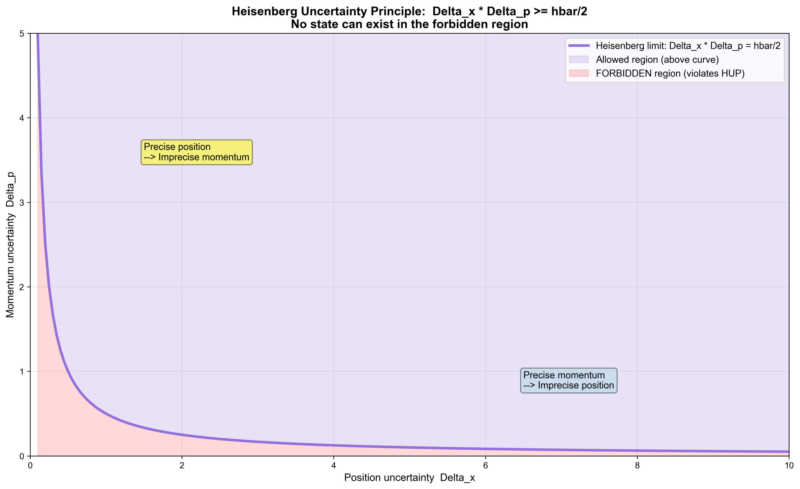
This insight shook him to his core. A few months later, he wrote down the famous uncertainty principle:
Δx · Δp ≥ ℏ/2
Where:
– Δx = uncertainty in position
– Δp = uncertainty in momentum
– ℏ = reduced Planck constant (1.055×10⁻³⁴ J·s)
This formula contains just five symbols, yet it overturned two millennia of assumptions about the nature of reality.
In his 1976 memoir, Heisenberg recalled:
“That night, I understood for the first time: nature is far more profound than any philosophy we have devised.”
The Uncertainty Principle: Not “We Can’t Measure It” — It’s “It Doesn’t Exist”
A Common Misconception
Many people think the uncertainty principle says:
“Our measurement instruments aren’t precise enough, so we can’t measure accurately.”
Wrong.
What Heisenberg actually said is:
“The particle itself does not possess simultaneously well-defined position and momentum.”
This is not an epistemological problem — a question about what we can know.
It is an ontological one — a question about what the world is.
Mathematical Derivation: From Commutation Relations to Uncertainty
In quantum mechanics, position x̂ and momentum p̂ are operators, not ordinary numbers.
They obey the commutation relation:
[x̂, p̂] = x̂p̂ – p̂x̂ = iℏ
This means: the order in which you measure position and momentum affects the result.
If x̂ and p̂ commuted (i.e., [x̂, p̂] = 0), they could have well-defined values simultaneously.
But they don’t commute ([x̂, p̂] = iℏ ≠ 0), so they cannot have well-defined values at the same time.
From the commutation relation, one can rigorously derive:
Δx · Δp ≥ ℏ/2
This is a mathematical theorem, not experimental error.
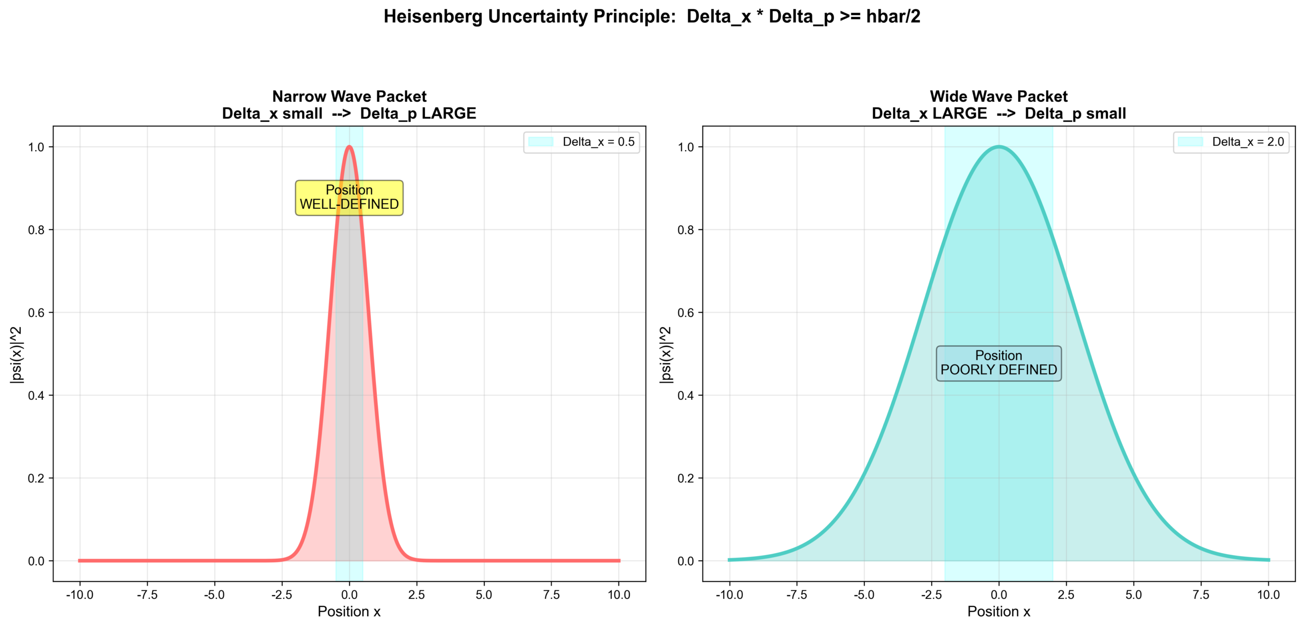
Physical Meaning: Wave Packets
From the perspective of wave mechanics, a particle is a wave packet.
The mathematical form of a wave packet:
ψ(x) = ∫ A(k) e^(ikx) dk
Where k = 2π/λ is the wave number, related to momentum by p = ℏk.
The spatial width Δx of the wave packet and the wave-number spread Δk satisfy:
Δx · Δk ≥ 1/2
Converting to momentum:
Δx · Δp ≥ ℏ/2
The physical picture:
– Δx small (position well-defined) → requires many different wavelengths (Δk large) superposed → momentum uncertain (Δp large)
– Δk small (momentum well-defined) → the wave packet spreads out in space (Δx large) → position uncertain
You cannot make a wave packet both narrow (well-defined position) and spectrally pure (well-defined momentum) at the same time.
This is not a technological limitation — it is a mathematical property of waves.
Other Uncertainty Relations
It’s not just position and momentum. Any two non-commuting observables have an uncertainty relation:
- Energy-time: ΔE · Δt ≥ ℏ/2
- Angular momentum components: Δ L_x · Δ L_y ≥ ℏ/2 |⟨L_z⟩|
- Spin components: Δ S_x · Δ S_y ≥ ℏ/2 |⟨S_z⟩|
General form:
Δ A · Δ B ≥ (1/2) |⟨[Â, B̂]⟩|
If two physical quantities don’t commute, they cannot be simultaneously well-defined.
Buddhist “Emptiness”: Nothing Has an Inherent Nature
2nd century CE, India.
The philosopher Nāgārjuna founded the Madhyamaka (“Middle Way”) school of Mahāyāna Buddhism. His central thesis was:
All phenomena are empty of inherent nature (svabhāva).
From the Mūlamadhyamakakārikā (“Fundamental Verses on the Middle Way”):
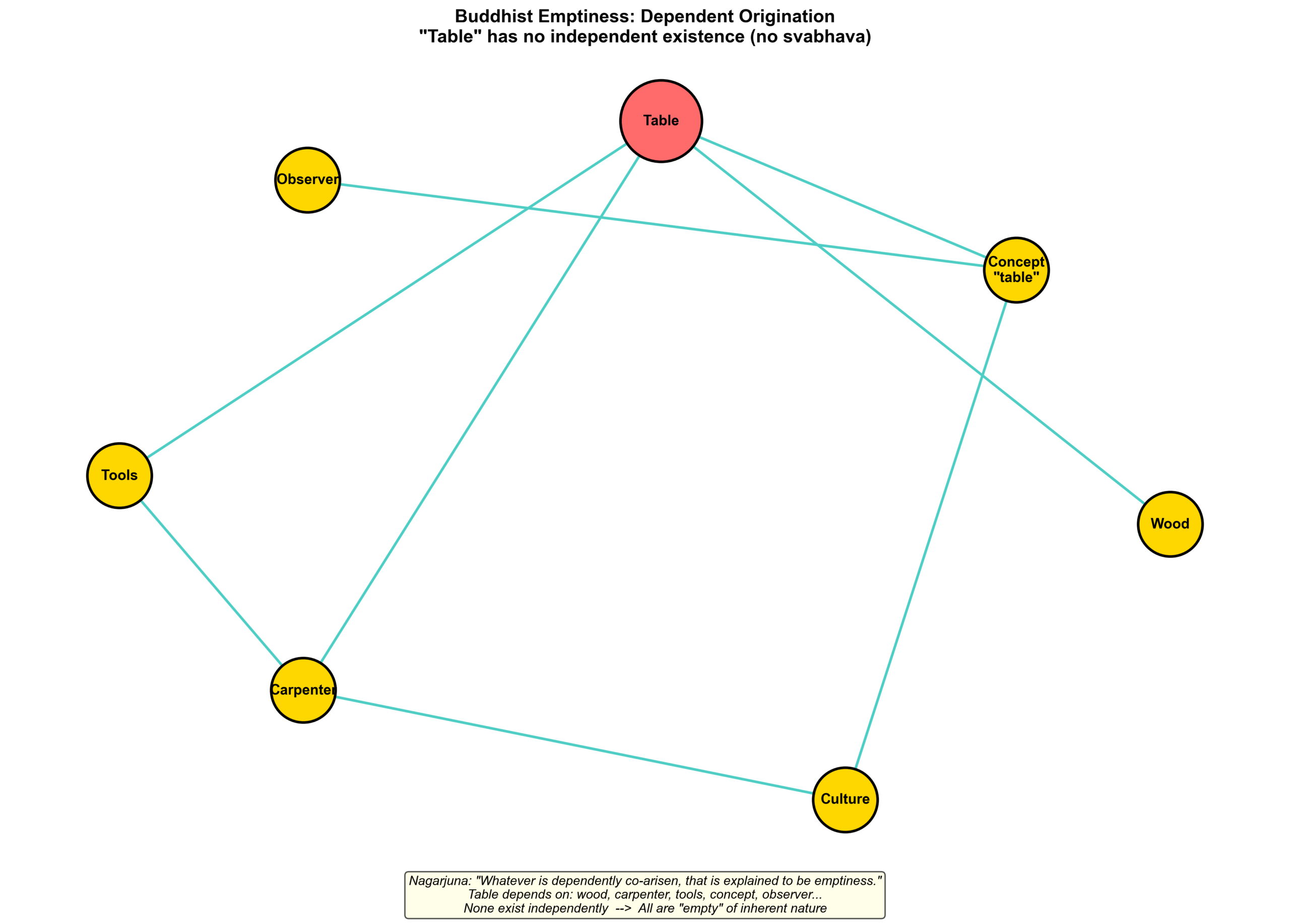
“Whatever is dependently co-arisen, that is explained to be emptiness.”
But what exactly does “emptiness” (Śūnyatā) mean? For Western readers more accustomed to the philosophical traditions of Plato and Aristotle — where things possess inherent “essences” or “Forms” — this concept can feel deeply counterintuitive. Let’s unpack it carefully.
A Common Misconception
Many people assume “emptiness” means:
“Nothing exists. The world is an illusion.”
Wrong.
What Nāgārjuna meant by “emptiness” is:
“No thing has an independent, self-existing essence (svabhāva).”
This is not nihilism — claiming nothing exists.
It is dependent origination (pratītyasamutpāda) — claiming everything exists in dependence on conditions.
Think of it this way: nihilism says the glass is empty because there’s no glass. Emptiness says the glass is real, but there’s no “essence of glass-ness” hiding inside it.
What is “Inherent Nature” (Svabhāva)?
Svabhāva refers to a hypothetical property that would be:
1. Independent — existing without relying on anything else
2. Immutable — unchanging regardless of conditions
3. Self-defining — definable without reference to relationships
Buddhism says: no phenomenon possesses svabhāva.
If this sounds abstract, consider an analogy from Western philosophy. Plato believed that a chair participates in the eternal “Form of Chair-ness.” Nāgārjuna would counter: there is no Form of Chair-ness. A chair is just wood, nails, a carpenter’s intention, and a human convention of naming — all the way down.
Three Layers of “Emptiness”
1. Emptiness Is Not Nothingness
The Heart Sutra — perhaps the most famous text in Mahāyāna Buddhism, recited daily by millions across East Asia — declares:
“Form is not different from emptiness;
Emptiness is not different from form.
Form is emptiness; emptiness is form.”
Here:
– Form (rūpa) = material phenomena, physical things
– Emptiness (śūnyatā) = the absence of inherent nature
The meaning:
– Physical things are inseparable from emptiness (form is not different from emptiness)
– Emptiness is inseparable from physical things (emptiness is not different from form)
– Physical things are emptiness (form is emptiness)
– Emptiness is physical things (emptiness is form)
Emptiness doesn’t mean “nothing is there.” It means “what’s there has no fixed, independent essence.”
2. Emptiness Is Dependent Origination
Nāgārjuna wrote: “Emptiness is dependent origination; dependent origination is emptiness.”
Dependent origination (pratītyasamutpāda) means: everything arises because of conditions, and changes when conditions change.
A familiar example: consider a table. It depends on wood, nails, a carpenter, tools, a design… Even the concept “table” depends on human habits of categorization. There is no independently existing “table-essence.”
If the table had “inherent nature,” it would:
– Not depend on wood (but it does)
– Never change (but it decays)
– Need no conditions to exist (but it had to be built)
Therefore, the table is “empty” — it has no svabhāva.
3. Emptiness Dissolves Attachment
Buddhism teaches that the root of suffering is attachment (upādāna) — clinging to things as if they were permanent and self-existing.
We cling to:
– The idea that “I” have a fixed essence → attachment to self
– The idea that things have fixed essences → attachment to phenomena
The wisdom of emptiness dissolves attachment:
– “I” is a convergence of causes and conditions — there is no independent “I”
– All things arise from causes and conditions — nothing has a permanent “essence”
Understanding emptiness is not a descent into nihilism. It is liberation — letting go of the illusion of fixedness.
A Striking Parallel: Uncertainty vs Emptiness
Let’s place the two frameworks side by side:
| Uncertainty Principle | Buddhist Emptiness |
|---|---|
| No fixed properties | No inherent nature (svabhāva) |
| A particle has no simultaneously well-defined position and momentum | No phenomenon has an independent, self-existing essence |
| Not “it has them but we can’t measure” | Not “it exists but we can’t see it” |
| Rather, “they genuinely don’t exist simultaneously” | Rather, “it genuinely has no fixed essence” |
| Properties depend on measurement | Existence depends on conditions |
| Position depends on how you measure | Nature depends on the angle of observation |
| Change the measurement, change the property | Change the conditions, change the quality |
| Commutation relations | Dependent origination |
| [x̂, p̂] = iℏ ≠ 0 | “This arising, that arises” |
| Position and momentum constrain each other | All things condition each other |
| No independent reality | No inherent nature |
| A particle is not “a little ball with a position” | A thing is not “an entity with an essence” |
Structural Correspondence, Not Superficial Analogy
Let’s be clear: this is not saying “quantum mechanics proves Buddhism is right.”
Rather, both point toward a reality that transcends fixed essences.
- Quantum mechanics discovered through experiment: properties are not intrinsic — they are products of measurement
- Buddhism discovered through contemplation: essences are not intrinsic — they are products of conditions
Both are saying: fixedness is not a fundamental feature of reality.
Indra’s Net: Everything Conditions Everything
The Avataṃsaka Sūtra (Flower Garland Sutra), a foundational text of the Huayan school of Buddhism, describes a stunning image called Indra’s Net:
In the heavenly palace of the god Indra, there hangs an infinite net. At every intersection of the net sits a jewel. Each jewel reflects every other jewel. And each reflection contains within it the reflections of all the other jewels. This goes on infinitely — an endless web of mutual reflection.
If you’ve ever stood between two facing mirrors and seen the infinite corridor of reflections, you’ve glimpsed a small piece of Indra’s Net.
The meaning:
– There is an infinite web of jewels
– Each jewel reflects all the others
– Each reflection contains all the other reflections
– Infinite recursion, mutual illumination
Philosophical implications:
– No jewel is independent (each contains the entire net)
– Change one jewel, and every jewel changes
– The part contains the whole; the whole contains the part
– One is all, and all is one
Quantum Entanglement: A Modern Indra’s Net
In quantum mechanics, two particles can exist in an entangled state:
|ψ⟩ = (|↑↓⟩ – |↓↑⟩) / √2
Properties of the entangled state:
– Particle A and Particle B are inseparable
– Measuring A instantly affects B (even if they’re light-years apart)
– A’s state cannot be defined independently
– The whole is greater than the sum of its parts
The parallels to Indra’s Net are remarkable:
– Each particle “reflects” the state of the other
– Changing one particle affects the entire system
– No particle has an independent state
Bell’s inequality (1964) and Aspect’s experiments (1982) proved:
Quantum entanglement is real — not explainable by hidden variables.
The 2022 Nobel Prize in Physics was awarded for precisely these entanglement experiments.
Python Models: Watching “Uncertainty” Emerge
Model 1: The Uncertainty Principle — An Interactive Experiment
First, we import the necessary scientific computing libraries and build the core class for the uncertainty principle. The Gaussian wave packet is the most commonly used wave function in quantum mechanics — it lets us directly see the tug-of-war between “well-defined position” and “well-defined momentum.”
import numpy as np
import matplotlib.pyplot as plt
from scipy.fft import fft, fftfreq

# Font configuration
plt.rcParams['font.sans-serif'] = ['Arial', 'Helvetica']
plt.rcParams['axes.unicode_minus'] = False

class UncertaintyPrinciple:
    """
    Uncertainty Principle Interactive Experiment
    Demonstrates: the trade-off between position uncertainty and momentum uncertainty
    """

    def __init__(self):
        self.hbar = 1.0  # Reduced Planck constant (arbitrary units)

    def gaussian_wavepacket(self, x, x0, sigma_x, k0):
        """
        Gaussian wave packet
        x0: center position
        sigma_x: position standard deviation (uncertainty)
        k0: center wave number (corresponding momentum p0 = hbar * k0)
        """
        return (1 / (2 * np.pi * sigma_x**2)**0.25) * \
               np.exp(-((x - x0)**2) / (4 * sigma_x**2)) * \
               np.exp(1j * k0 * x)

    def momentum_distribution(self, psi_x, dx):
        """
        Compute momentum-space wave function from position-space wave function
        using Fourier transform
        """
        psi_k = fft(psi_x) * dx
        return psi_k
Next comes the heart of the visualization: we generate wave packets for four different sigma_x values, then use the Fourier transform to obtain the corresponding momentum distributions. The key insight in this code is that when the wave packet is narrower in position space (small Δx), it becomes wider in momentum space (large Δp), and vice versa. This is not a numerical artifact — it is a mathematical necessity of the Fourier transform.
    def visualize_uncertainty(self, sigma_x_values=[0.5, 1.0, 2.0, 4.0]):
        """
        Visualize wave packets with different position uncertainties
        """
        x = np.linspace(-20, 20, 2000)
        dx = x[1] - x[0]

        fig, axes = plt.subplots(2, len(sigma_x_values), figsize=(18, 10))

        for i, sigma_x in enumerate(sigma_x_values):
            # Generate wave packet
            psi_x = self.gaussian_wavepacket(x, x0=0, sigma_x=sigma_x, k0=5)

            # Position-space probability density
            prob_x = np.abs(psi_x)**2

            # Momentum space
            psi_k = self.momentum_distribution(psi_x, dx)
            k = fftfreq(len(x), dx) * 2 * np.pi
            prob_k = np.abs(psi_k)**2

            # Reorder (fft output needs rearranging)
            k_sorted_idx = np.argsort(k)
            k_sorted = k[k_sorted_idx]
            prob_k_sorted = prob_k[k_sorted_idx]

            # Calculate uncertainties
            delta_x = sigma_x
            delta_k = 1 / (2 * sigma_x)
            delta_p = self.hbar * delta_k
            uncertainty_product = delta_x * delta_p
Each set of wave packets produces two plots: the top row shows the position-space probability density (blue), and the bottom row shows the momentum-space probability density (red). Notice that the uncertainty product Δx·Δp is always greater than or equal to ℏ/2 — this is the mathematical embodiment of Heisenberg’s uncertainty principle.
            # === Top row: Position space ===
            ax = axes[0, i]
            ax.plot(x, prob_x, 'b-', linewidth=2)
            ax.fill_between(x, 0, prob_x, alpha=0.3, color='blue')
            ax.set_xlabel('Position x', fontsize=11)
            ax.set_ylabel('|ψ(x)|²', fontsize=11)
            ax.set_title(f'Position Uncertainty\nΔx = {delta_x:.2f}',
                        fontsize=12, fontweight='bold', color='blue')
            ax.grid(True, alpha=0.3)
            ax.set_xlim(-15, 15)
            ax.axvspan(-delta_x, delta_x, alpha=0.2, color='cyan',
                      label=f'Δx = {delta_x:.2f}')
            ax.legend(fontsize=9)

            # === Bottom row: Momentum space ===
            ax = axes[1, i]
            center_idx = len(k_sorted) // 2
            plot_range = 500
            k_plot = k_sorted[center_idx-plot_range:center_idx+plot_range]
            prob_k_plot = prob_k_sorted[center_idx-plot_range:center_idx+plot_range]

            if np.max(prob_k_plot) > 0:
                prob_k_plot = prob_k_plot / np.max(prob_k_plot)

            ax.plot(k_plot, prob_k_plot, 'r-', linewidth=2)
            ax.fill_between(k_plot, 0, prob_k_plot, alpha=0.3, color='red')
            ax.set_xlabel('Wave number k (momentum p=ℏk)', fontsize=11)
            ax.set_ylabel('|ψ(k)|²', fontsize=11)
            ax.set_title(f'Momentum Uncertainty\nΔp = {delta_p:.2f}',
                        fontsize=12, fontweight='bold', color='red')
            ax.grid(True, alpha=0.3)

            color = 'green' if uncertainty_product >= self.hbar/2 else 'red'
            ax.text(0.5, 0.9,
                   f'Δx·Δp = {uncertainty_product:.3f}\n(ℏ/2 = {self.hbar/2:.3f})',
                   transform=ax.transAxes, ha='center', fontsize=10,
                   bbox=dict(boxstyle='round', facecolor=color, alpha=0.5))

        fig.text(0.5, 0.98, 'Uncertainty Principle: Smaller Δx → Larger Δp',
                ha='center', fontsize=16, fontweight='bold')
        fig.text(0.5, 0.02,
                'Key Insight: This is not measurement error — it is a mathematical property of waves!\n'
                'You cannot make a wave packet both narrow (well-defined position) and spectrally pure (well-defined momentum)',
                ha='center', fontsize=11,
                bbox=dict(boxstyle='round', facecolor='yellow', alpha=0.5))

        plt.tight_layout()
        plt.subplots_adjust(top=0.93, bottom=0.1)
        plt.savefig('uncertainty_principle_visualization.png', dpi=300, bbox_inches='tight')
        plt.show()
The final segment produces text output for an interactive measurement experiment. It simulates two scenarios — “measure position first, then momentum” and “measure momentum first, then position” — revealing that the order of measurement fundamentally changes the result, because the position and momentum operators don’t commute. This also introduces the Buddhist analogy: nothing has a fixed “inherent nature”; properties manifest depending on how we observe.
    def interactive_measurement(self):
        """
        Interactive measurement: observe the effect of measurement order
        """
        print("\n" + "="*70)
        print("  UNCERTAINTY PRINCIPLE — INTERACTIVE EXPERIMENT")
        print("="*70)

        x = np.linspace(-10, 10, 1000)
        sigma_x = 1.0
        psi = self.gaussian_wavepacket(x, x0=0, sigma_x=sigma_x, k0=5)

        print("\nInitial state:")
        print(f"  Position uncertainty  Δx ≈ {sigma_x:.2f}")
        print(f"  Momentum uncertainty  Δp ≈ {self.hbar/(2*sigma_x):.2f}")
        print(f"  Uncertainty product   Δx·Δp ≈ {sigma_x * self.hbar/(2*sigma_x):.3f}")
        print(f"  Heisenberg lower bound ℏ/2 = {self.hbar/2:.3f}")

        print("\nExperiment 1: Measure position first, then momentum")
        print("  → After measuring position, the wave function collapses to a point")
        print("  → Now Δx → 0, therefore Δp → ∞")
        print("  → Momentum becomes completely uncertain!")

        print("\nExperiment 2: Measure momentum first, then position")
        print("  → After measuring momentum, the wave function becomes a plane wave")
        print("  → Now Δp → 0, therefore Δx → ∞")
        print("  → Position becomes completely uncertain!")

        print("\nConclusion:")
        print("  • Measurement order matters (x̂ and p̂ don't commute)")
        print("  • Measuring one quantity disturbs the other")
        print("  • This is not an instrument problem — it is a law of nature")

        print("\nBuddhist parallel:")
        print("  • Nothing has a fixed 'inherent nature'")
        print("  • Properties depend on how we observe")
        print("  • Different perspectives reveal different aspects")
        print("="*70)

# Run
experiment = UncertaintyPrinciple()
experiment.visualize_uncertainty(sigma_x_values=[0.5, 1.0, 2.0, 4.0])
experiment.interactive_measurement()
Output:
– 4 comparison plots showing different Δx values and their corresponding Δp
– Clear visual: when Δx is small, Δp is large; when Δx is large, Δp is small
– The uncertainty product Δx·Δp always ≥ ℏ/2
Key Insight:
This is not “imprecise measurement.” It is a mathematical property of waves.
If you want a narrow wave packet (well-defined position), you must superpose many wavelengths (uncertain momentum).
Model 2: Visualizing “Emptiness” — Properties Depend on Conditions
This model uses everyday experience to visualize the concept of “emptiness.” We take a cup as an example: viewed from above, it appears circular; viewed from the side, it appears rectangular. What is the “true shape” of the cup? The answer is — there is no “fixed shape” independent of the viewing angle.
def visualize_emptiness():
    """
    Visualizing 'Emptiness'
    Demonstrates: how an object's properties depend on the conditions of observation
    """

    fig = plt.figure(figsize=(16, 12))

    # === Example: The "Emptiness" of a Cup ===

    # Subplot 1: Different angles reveal different shapes
    ax1 = fig.add_subplot(2, 3, 1)
    circle = plt.Circle((0.5, 0.5), 0.3, fill=False, edgecolor='blue', linewidth=3)
    ax1.add_patch(circle)
    ax1.text(0.5, 0.1, 'Top view: Circle', ha='center', fontsize=12, fontweight='bold')
    ax1.set_xlim(0, 1)
    ax1.set_ylim(0, 1)
    ax1.set_aspect('equal')
    ax1.axis('off')

    # Subplot 2: Side view: rectangle
    ax2 = fig.add_subplot(2, 3, 2)
    rect = plt.Rectangle((0.2, 0.2), 0.6, 0.6, fill=False, edgecolor='red', linewidth=3)
    ax2.add_patch(rect)
    ax2.text(0.5, 0.1, 'Side view: Rectangle', ha='center', fontsize=12, fontweight='bold')
    ax2.set_xlim(0, 1)
    ax2.set_ylim(0, 1)
    ax2.set_aspect('equal')
    ax2.axis('off')

    # Subplot 3: The question
    ax3 = fig.add_subplot(2, 3, 3)
    ax3.text(0.5, 0.5, 'Q: What is the cup\'s\n"true shape"?\n\nA: There is no\n"fixed shape"!\n\nShape depends on\nthe viewing angle',
            ha='center', va='center', fontsize=13,
            bbox=dict(boxstyle='round', facecolor='yellow', alpha=0.7))
    ax3.set_xlim(0, 1)
    ax3.set_ylim(0, 1)
    ax3.axis('off')
The bottom row extends the same logic to the quantum world. Measuring “position” yields one distribution; measuring “momentum” yields another — the particle’s “true state” likewise has no fixed answer independent of the measurement. This is the structural correspondence between emptiness and the uncertainty principle.
    # === Quantum analogy: The "position" of a particle ===

    # Subplot 4: Position measurement
    ax4 = fig.add_subplot(2, 3, 4)
    x = np.linspace(-5, 5, 1000)
    psi_position = np.exp(-x**2)
    ax4.plot(x, psi_position, 'b-', linewidth=3)
    ax4.fill_between(x, 0, psi_position, alpha=0.3, color='blue')
    ax4.set_xlabel('Position', fontsize=11)
    ax4.set_ylabel('Probability', fontsize=11)
    ax4.set_title('Measure "Position"\n→ Position well-defined', fontsize=12, fontweight='bold', color='blue')
    ax4.grid(True, alpha=0.3)

    # Subplot 5: Momentum measurement
    ax5 = fig.add_subplot(2, 3, 5)
    k = np.linspace(-5, 5, 1000)
    psi_momentum = np.exp(-(k-2)**2/4)
    ax5.plot(k, psi_momentum, 'r-', linewidth=3)
    ax5.fill_between(k, 0, psi_momentum, alpha=0.3, color='red')
    ax5.set_xlabel('Momentum', fontsize=11)
    ax5.set_ylabel('Probability', fontsize=11)
    ax5.set_title('Measure "Momentum"\n→ Momentum well-defined', fontsize=12, fontweight='bold', color='red')
    ax5.grid(True, alpha=0.3)

    # Subplot 6: Conclusion
    ax6 = fig.add_subplot(2, 3, 6)
    ax6.text(0.5, 0.5, 'Q: What is the particle\'s\n"true state"?\n\nA: There are no\n"fixed properties"!\n\nProperties depend on\nthe measurement',
            ha='center', va='center', fontsize=13,
            bbox=dict(boxstyle='round', facecolor='lightblue', alpha=0.7))
    ax6.set_xlim(0, 1)
    ax6.set_ylim(0, 1)
    ax6.axis('off')
Finally, we add titles, annotations, and print the three layers of emptiness in parallel. The output here is especially worth noting: it places the Buddhist concept of “dependent origination” and quantum “measurement dependence” into the same framework — the world is not made of “objects with fixed properties,” but of “relationships that manifest under conditions.”
    # Title and comparison notes
    fig.text(0.5, 0.98, 'Structural Parallel: "Emptiness" and "Uncertainty"',
            ha='center', fontsize=16, fontweight='bold')
    fig.text(0.5, 0.02,
            'Buddhism: Things have no "inherent nature" (fixed essence) — properties manifest depending on conditions\n'
            'Quantum Mechanics: Particles have no "definite properties" — properties are determined by measurement\n'
            'Common ground: "Fixedness" is not a fundamental feature of reality',
            ha='center', fontsize=11,
            bbox=dict(boxstyle='round', facecolor='lightyellow', alpha=0.7))

    plt.tight_layout()
    plt.subplots_adjust(top=0.93, bottom=0.12)
    plt.savefig('emptiness_visualization.png', dpi=300, bbox_inches='tight')
    plt.show()

    # Text explanation
    print("\n" + "="*70)
    print("  THREE LAYERS OF EMPTINESS")
    print("="*70)

    print("\n1. Emptiness Is Not Nothingness")
    print("   Heart Sutra: 'Form is emptiness; emptiness is form'")
    print("   → Things exist, but they have no fixed essence")

    print("\n2. Emptiness Is Dependent Origination")
    print("   Nagarjuna: 'Whatever is dependently co-arisen is explained to be emptiness'")
    print("   → Everything exists in dependence on conditions")

    print("\n3. Emptiness Dissolves Attachment")
    print("   → There is no fixed 'self'")
    print("   → There are no fixed 'things'")
    print("   → Realizing emptiness, we let go of clinging")

    print("\nParallel with the Uncertainty Principle:")
    print("   • A particle has no fixed 'position' or 'momentum'")
    print("   • Properties depend on the method of measurement")
    print("   • There are no 'objective properties' independent of observation")

    print("\nShared insight:")
    print("   The world is not composed of 'objects with fixed properties'")
    print("   but of 'relationships that manifest under conditions'")
    print("="*70)

# Run
visualize_emptiness()
Output:
– Top row: A cup seen from different angles reveals different shapes
– Bottom row: Measuring a particle’s position vs momentum yields different results
– Visualizes “properties depend on observation”
Philosophical insight:
Buddhism: properties depend on the angle of observation
Quantum mechanics: properties depend on the method of measurement
Common ground: there are no fixed properties independent of observation
Model 3: Indra’s Net — Visualizing Quantum Entanglement
This model uses NetworkX to build two side-by-side networks: one representing the Huayan school’s Indra’s Net (a 2D grid), the other representing a quantum entanglement network (3D randomly distributed particles). The red-highlighted node represents the “jewel that was changed” — in Indra’s Net, changing one jewel changes the reflections of the entire web; in quantum entanglement, measuring one particle instantly affects all entangled particles.
import networkx as nx
from mpl_toolkits.mplot3d import Axes3D

def indras_net_quantum():
    """
    Indra's Net and Quantum Entanglement
    Demonstrates: everything is interconnected — changing one affects all
    """

    fig = plt.figure(figsize=(18, 12))

    # === Left plot: Indra's Net (2D network) ===
    ax1 = fig.add_subplot(2, 2, 1)

    n = 5
    G = nx.grid_2d_graph(n, n)
    pos = {(i, j): (i, j) for i, j in G.nodes()}

    nx.draw_networkx_nodes(G, pos, node_color='gold', node_size=800,
                          edgecolors='black', linewidths=2, ax=ax1)
    nx.draw_networkx_edges(G, pos, edge_color='gray', width=2, ax=ax1)

    highlight_node = (2, 2)
    nx.draw_networkx_nodes(G, pos, nodelist=[highlight_node],
                          node_color='red', node_size=1000,
                          edgecolors='black', linewidths=3, ax=ax1)

    ax1.set_title("Indra's Net: Each jewel reflects all others\nChange one, and every reflection changes",
                 fontsize=13, fontweight='bold')
    ax1.axis('off')
    ax1.text(2, -0.5, 'Huayan Buddhism: One is all, and all is one',
            ha='center', fontsize=11,
            bbox=dict(boxstyle='round', facecolor='lightyellow', alpha=0.7))

    # === Right plot: Quantum entanglement network (3D) ===
    ax2 = fig.add_subplot(2, 2, 2, projection='3d')

    n_particles = 8
    positions = np.random.randn(n_particles, 3)

    ax2.scatter(positions[:, 0], positions[:, 1], positions[:, 2],
               c='cyan', s=300, edgecolors='black', linewidth=2, alpha=0.8)

    for i in range(n_particles):
        for j in range(i+1, n_particles):
            ax2.plot([positions[i, 0], positions[j, 0]],
                    [positions[i, 1], positions[j, 1]],
                    [positions[i, 2], positions[j, 2]],
                    'b-', alpha=0.2, linewidth=1)

    ax2.scatter([positions[0, 0]], [positions[0, 1]], [positions[0, 2]],
               c='red', s=500, edgecolors='black', linewidth=3, zorder=10)

    ax2.set_title('Quantum Entanglement: Non-local correlations\nMeasure one particle, affect them all',
                 fontsize=13, fontweight='bold')
    ax2.set_xlabel('X')
    ax2.set_ylabel('Y')
    ax2.set_zlabel('Z')
The two bottom subplots present the mathematical structure and philosophical parallels in text boxes. The lower left lists the Bell state formulas and the experimental history of Bell inequality violations; the lower right lines up the features of Indra’s Net and quantum entanglement in a point-by-point comparison. Their shared conclusion: the world is not “a collection of independent entities,” but “an interdependent web of relationships.”
    # === Bottom left: Entangled state mathematics ===
    ax3 = fig.add_subplot(2, 2, 3)
    ax3.axis('off')

    text = '''
    Entangled State (Bell State):

    |ψ⟩ = (|↑↓⟩ - |↓↑⟩) / √2

    Properties:
    • Particles A and B are inseparable
    • Measure A → instantly know B
    • A's state cannot be defined alone
    • The whole ≠ sum of parts

    Bell's Inequality (1964):
    If particles have "local realism"
    → a certain inequality must hold

    Experimental results (1982-2022):
    The inequality is violated!
    → No local realism
    → Entanglement is real
    '''

    ax3.text(0.1, 0.5, text, fontsize=11, va='center', family='monospace',
            bbox=dict(boxstyle='round', facecolor='lightblue', alpha=0.7))

    # === Bottom right: Indra's Net vs Entanglement ===
    ax4 = fig.add_subplot(2, 2, 4)
    ax4.axis('off')

    comparison = '''
    Indra's Net vs Quantum Entanglement

    Indra's Net:
    • Each jewel contains the entire net
    • Change one jewel, the whole net shifts
    • The part is the whole
    • One is all

    Quantum Entanglement:
    • Each particle carries information about the whole system
    • Measure one particle, affect all entangled partners
    • Individual particle states cannot be defined alone
    • The whole is irreducible

    Common ground:
    → No truly "independent" parts
    → Everything is interdependent
    → Changing a part = changing the whole
    '''

    ax4.text(0.1, 0.5, comparison, fontsize=11, va='center',
            bbox=dict(boxstyle='round', facecolor='lightyellow', alpha=0.7))

    plt.tight_layout()
    plt.savefig('indras_net_entanglement.png', dpi=300, bbox_inches='tight')
    plt.show()
The final text output weaves together historical timelines and philosophical insights — from the Avataṃsaka Sūtra to Aspect’s experiments, from the 2022 Nobel Prize to Buddhist dependent origination.
    # Detailed text output
    print("\n" + "="*70)
    print("  INDRA'S NET AND QUANTUM ENTANGLEMENT")
    print("="*70)

    print("\nIndra's Net (from the Avatamsaka Sutra):")
    print("  • An infinite net of jewels")
    print("  • Each jewel reflects every other jewel")
    print("  • Infinite recursion, mutual illumination")
    print("  → One is all, and all is one")

    print("\nQuantum Entanglement:")
    print("  • Two or more particles exist in an entangled state")
    print("  • |ψ⟩ = (|↑↓⟩ - |↓↑⟩) / √2")
    print("  • Measuring one particle instantly affects its partners")
    print("  • Correlations persist even across light-years")

    print("\nExperimental evidence:")
    print("  • 1982: Aspect's experiment confirms entanglement")
    print("  • 2015: 'Loophole-free' Bell tests")
    print("  • 2022: Nobel Prize in Physics")

    print("\nPhilosophical implications:")
    print("  • No particle is truly 'independent'")
    print("  • The universe is an indivisible whole")
    print("  • 'Separation' is an illusion")

    print("\nBuddhist 'Dependent Origination':")
    print("  • 'This arising, that arises; this ceasing, that ceases'")
    print("  • All phenomena mutually condition one another")
    print("  • There is no independently existing 'self' or 'thing'")

    print("\nShared insight:")
    print("  The world is not 'a collection of independent entities'")
    print("  but 'an interdependent web of relationships'")
    print("="*70)

# Run
indras_net_quantum()
Output:
– Four plots showing the parallels between Indra’s Net and quantum entanglement
– 2D network + 3D entanglement visualization
– Mathematical formulas + comparison table
Profound insight:
The cosmic structure described by Huayan Buddhism 1,500 years ago through Indra’s Net is strikingly similar to the non-local correlations revealed by quantum entanglement.
Model 4: The “Emptiness” of Self — The Self as an Entangled State
This model visualizes the Buddhist concept of “no-self” (anātman) through two contrasting diagrams. The left panel shows our habitual “classical view of self”: a red “Self” at the center, surrounded by family, friends, work, body, memories, and thoughts — as if “I” were an independent core that possesses all of these.
def self_as_entanglement():
    """
    The 'Emptiness' of Self
    Demonstrates: how the 'self' is a convergence of causes and conditions,
    with no independent inherent nature
    """

    fig, (ax1, ax2) = plt.subplots(1, 2, figsize=(16, 8))

    # === Left panel: The classical notion of "self" ===
    circle_self = plt.Circle((0.5, 0.5), 0.15, color='red', alpha=0.7,
                            edgecolor='black', linewidth=3)
    ax1.add_patch(circle_self)
    ax1.text(0.5, 0.5, 'Self', ha='center', va='center', fontsize=20,
            fontweight='bold', color='white')

    external_things = [
        (0.2, 0.8, 'Family'),
        (0.8, 0.8, 'Friends'),
        (0.1, 0.5, 'Work'),
        (0.9, 0.5, 'Body'),
        (0.2, 0.2, 'Memories'),
        (0.8, 0.2, 'Thoughts'),
    ]

    for x, y, label in external_things:
        circle = plt.Circle((x, y), 0.08, color='lightblue', alpha=0.5,
                           edgecolor='gray', linewidth=1.5)
        ax1.add_patch(circle)
        ax1.text(x, y, label, ha='center', va='center', fontsize=10)
        ax1.annotate('', xy=(x, y), xytext=(0.5, 0.5),
                    arrowprops=dict(arrowstyle='->', lw=1.5, color='black', alpha=0.5))

    ax1.set_xlim(0, 1)
    ax1.set_ylim(0, 1)
    ax1.set_aspect('equal')
    ax1.axis('off')
    ax1.set_title('Classical View: An Independent "Self"\n"I" possess body, memories, thoughts...',
                 fontsize=14, fontweight='bold')
    ax1.text(0.5, 0.05, 'Assumption: there exists an independent "self" at the core',
            ha='center', fontsize=11,
            bbox=dict(boxstyle='round', facecolor='lightcoral', alpha=0.7))
The right panel presents the Buddhist view of the “Five Aggregates” (skandhas): no center, just five interconnected elements — form, feeling, perception, volition, and consciousness. The “self” is not an independent entity but a temporary pattern arising from their convergence — just as a particle is not an independent “little ball” but an excitation pattern of a field.
    # === Right panel: Buddhist "No-Self" (Anātman) ===
    elements = [
        (0.3, 0.7, 'Form'),
        (0.7, 0.7, 'Feeling'),
        (0.5, 0.5, 'Perception'),
        (0.3, 0.3, 'Volition'),
        (0.7, 0.3, 'Consciousness'),
    ]

    for x, y, label in elements:
        circle = plt.Circle((x, y), 0.1, color='lightgreen', alpha=0.6,
                           edgecolor='green', linewidth=2)
        ax2.add_patch(circle)
        ax2.text(x, y, label, ha='center', va='center', fontsize=12,
                fontweight='bold')

    for i, (x1, y1, _) in enumerate(elements):
        for x2, y2, _ in elements[i+1:]:
            ax2.plot([x1, x2], [y1, y2], 'g-', alpha=0.3, linewidth=2)

    ax2.set_xlim(0, 1)
    ax2.set_ylim(0, 1)
    ax2.set_aspect('equal')
    ax2.axis('off')
    ax2.set_title('Buddhist View: The Five Aggregates — No-Self\nNo independent "I", only interdependent conditions',
                 fontsize=14, fontweight='bold')
    ax2.text(0.5, 0.05, 'Reality: "I" is a temporary convergence of Five Aggregates (form, feeling, perception, volition, consciousness)',
            ha='center', fontsize=11,
            bbox=dict(boxstyle='round', facecolor='lightgreen', alpha=0.7))

    plt.tight_layout()
    plt.savefig('self_emptiness.png', dpi=300, bbox_inches='tight')
    plt.show()
The text output draws a compelling analogy between the Five Aggregates and quantum state representations. A particle’s state can be expanded in different bases (position basis, momentum basis), and no basis is “the essential one” — likewise, the “self” can be understood from different angles (body, memory, environment), but none of them constitutes an independently existing “core self.”
    # Quantum analogy
    print("\n" + "="*70)
    print("  THE EMPTINESS OF SELF: THE SELF AS AN ENTANGLED STATE")
    print("="*70)

    print("\nThe Buddhist 'Five Aggregates' (skandhas):")
    print("  1. Form (rupa):         body, matter")
    print("  2. Feeling (vedana):    sensations")
    print("  3. Perception (samjna): concepts, recognition")
    print("  4. Volition (samskara): will, behavioral tendencies")
    print("  5. Consciousness (vijnana): awareness")

    print("\nBuddhist teaching:")
    print("  • There is no independent 'self'")
    print("  • 'Self' is merely a temporary configuration of the Five Aggregates")
    print("  • Aggregates converge → the illusion of 'self' arises")
    print("  • Aggregates disperse → 'self' disappears")

    print("\nQuantum analogy:")
    print("  • A particle has no independent 'state'")
    print("  • 'State' is a projection onto a measurement basis")
    print("  • A system can be decomposed into different bases:")
    print("    |ψ⟩ = Σ cᵢ|φᵢ⟩ (position basis)")
    print("    |ψ⟩ = Σ dⱼ|χⱼ⟩ (momentum basis)")
    print("  • No 'essential' state — only expressions relative to a basis")

    print("\nHow the 'self' resembles an entangled state:")
    print("  |self⟩ = α|body⟩|memory⟩|environment⟩... (simplified)")
    print("  ")
    print("  • 'Self' is entangled with body (change the body → 'self' changes)")
    print("  • 'Self' is entangled with memory (amnesia → 'self' changes)")
    print("  • 'Self' is entangled with environment (new context → 'self' changes)")
    print("  • There is no 'core self' independent of all these")

    print("\nPractical implications:")
    print("  • Clinging to a fixed 'self' is the root of suffering")
    print("  • Realizing 'no-self' can bring liberation")
    print("  • This does not mean 'I don't exist' — it means 'I have no fixed essence'")
    print("  • 'I' exists dependently — when conditions change, 'I' changes")

    print("\nA deep question:")
    print("  If 'I' has no inherent nature, then who is reading these words?")
    print("  Answer: The process of reading is happening, but there is no independent 'reader.'")
    print("  Just as wave function collapse happens, but there is no independent 'particle.'")
    print("="*70)

# Run
self_as_entanglement()
Output:
– Left panel: The classical notion of “self” (an independent “I”)
– Right panel: The Buddhist Five Aggregates (no independent “I”)
– Quantum analogy: how the “self” resembles an entangled state
The deepest insight:
The “self” is not an independent entity, but a temporary pattern arising from the convergence of body, mind, and environment.
Just as a particle is not an independent “little ball,” but an excitation pattern of a field.
Einstein’s Final Doubt
April 18, 1955. Einstein, days from death.
He wrote a final letter to a friend, discussing quantum mechanics:
“I cannot believe that God plays dice… Perhaps we simply haven’t found the deeper theory yet.”
Einstein never accepted the uncertainty of quantum mechanics.
He believed:
– There must be “hidden variables”
– Particles really do have definite position and momentum
– We just don’t know what they are
But he was wrong.
In 1964, John Bell derived “Bell’s inequality”:
– If hidden variables exist → experiments should satisfy a certain inequality
– Quantum mechanics predicts → the inequality is violated
From 1982 to 2022, experiment after experiment confirmed: the inequality is violated.
Conclusion: There are no hidden variables. Uncertainty is fundamental.
Einstein’s intuition — “reality should be deterministic” — was overturned by experiment.
What Would the Buddha Say?
If the Buddha had known about the uncertainty principle, he might have said:
“This is precisely what I meant by ‘no inherent nature.’
A particle has no fixed position or momentum, just as all things have no fixed essence.
Properties manifest depending on conditions, just as all phenomena arise depending on causes.
Uncertainty is not a flaw — it is the nature of reality.”
Questions for Reflection
-
Heisenberg says “a particle has no simultaneously well-defined position and momentum.” Does this contradict everyday experience? Why or why not?
-
If uncertainty is fundamental, where does “certainty” come from? Why does the macroscopic world appear deterministic?
-
Buddhism says “the self has no inherent nature.” Then who is realizing “no-self”? Is this a paradox?
-
Can quantum entanglement “prove” that everything is interdependent? Or is it merely an analogy?
-
If you accepted that “nothing has an inherent nature,” would it change how you live? How?
Conclusion
On that dawn when Heisenberg waited for sunrise on Helgoland, he glimpsed a truth that shook him: particles have no fixed properties.
2,500 years earlier, the philosopher Nāgārjuna in India wrote down an equally startling insight: nothing has a fixed essence.
They used different languages — one mathematics, the other philosophy. Their methods differed — one ran experiments, the other practiced deep contemplation.
But they pointed in the same direction:
“Fixedness” is not a fundamental feature of reality.
Uncertainty is not a defect. Emptiness is not nothingness.
Both describe a deeper structure of reality:
Everything exists in dependence on conditions, and manifests through relationships.
When we use Python to simulate the uncertainty of wave packets, when we visualize the no-self structure of the Five Aggregates, we are not merely doing an academic exercise.
We are experiencing a new way of seeing the world.
Perhaps this is exactly what Heisenberg meant: “Nature is far more profound than any philosophy we have devised.”
Next Article Preview
#05: Quantum Entanglement vs the Huayan Buddhist “Indra’s Net”
In 1935, Einstein published the EPR paper, attempting to prove that quantum mechanics was incomplete.
He called it “spooky action at a distance” and thought it was too absurd to be true.
But experiments proved: it is real.
In the next article, we will explore:
– The complete theory of quantum entanglement
– The EPR paradox and Bell’s inequality
– The 2022 Nobel Prize experiments
– Huayan Buddhism’s “Dharmadhātu dependent origination”
– Simulating non-local correlations of entangled particles with Python
References
- Heisenberg, W. (1927). “Uber den anschaulichen Inhalt der quantentheoretischen Kinematik und Mechanik”. Zeitschrift fur Physik, 43, 172-198.
- Nagarjuna (2nd century). Mulamadhyamakakarika.
- Heart Sutra (Prajnaparamita Hrdaya).
- Bell, J. S. (1964). “On the Einstein Podolsky Rosen Paradox”. Physics, 1(3), 195-200.
- Aspect, A., et al. (1982). “Experimental Realization of Einstein-Podolsky-Rosen-Bohm Gedankenexperiment”. Physical Review Letters, 49, 91-94.
- Avatamsaka Sutra.
- Griffiths, D. J. (2018). Introduction to Quantum Mechanics (3rd ed.). Cambridge University Press.