The Eve of the Quantum Revolution — When Newton’s Universe Began to Crumble
Series: Quantum Mechanics Meets Eastern Philosophy #01/12 | Reading time: 25 min | Python (NumPy, Matplotlib, SciPy)
Author: Wina @ Code & Cogito
An Act of Desperation
December 14, 1900. Berlin. A bitter winter wind swept down Wilhelmstrasse as a 42-year-old physicist stood before the German Physical Society, about to present a formula that would change the world.
His name was Max Planck.
His hands were trembling — not from stage fright, but from a quiet fury directed at himself. The formula he was about to unveil solved the “black-body radiation problem” that had stumped physicists for years. But it came at a price: he had to introduce an assumption he considered absurd.
“Energy is not continuous,” he told the audience, his voice measured and low. “It comes in discrete, indivisible packets.”
E = hv
This deceptively simple equation — where h (Planck’s constant, 6.626×10⁻³⁴ joule-seconds) was an entirely new fundamental quantity — would tear apart the cosmic order Isaac Newton had built.
After the lecture, Planck said something to his son that has become one of the most famous confessions in the history of science:
“It was an act of desperation. By nature I am peacefully inclined and reject all doubtful adventures… But I had wrestled with the problem for six years. I knew that it had to be solved, at whatever cost. I was ready to sacrifice every one of my previous convictions…”
Planck didn’t know it, but he had just lit the fuse of a revolution.
A revolution that would tell humanity: the world you think you know is not the real world.
The Grand Palace of Classical Physics
To appreciate just how seismic the quantum revolution was, we need to understand what it demolished.
Newton’s Clockwork Universe (1687–1900)
In 1687, Isaac Newton published the Philosophiae Naturalis Principia Mathematica — the Principia, for short. With three laws of motion and a law of universal gravitation, he explained everything from falling apples to orbiting planets.
Newton’s universe was a precision clockwork mechanism:
First Law (Inertia):
An object at rest stays at rest; an object in motion stays in motion — unless an external force intervenes.
Second Law (F = ma):
Force equals mass times acceleration. Give me the starting conditions, and I can calculate the trajectory of anything.
Third Law (Action and Reaction):
For every action, there is an equal and opposite reaction. The universe is symmetrical and predictable.
Law of Universal Gravitation:
F = G(m₁m₂)/r²
Every pair of objects in the universe attracts each other, and the force depends only on their masses and the distance between them.
The elegance of this framework was breathtaking. In 1758, Halley’s Comet returned right on schedule, exactly as Newton’s equations had predicted. In 1846, anomalies in the orbit of Uranus led mathematicians to calculate the position of Neptune — they knew where it was before anyone pointed a telescope at it.
By the end of the 19th century, physicists were becoming convinced: the fundamental laws of the universe had been found.
Laplace’s All-Knowing Demon
In 1814, the French mathematician Pierre-Simon Laplace articulated what may be the boldest declaration in the history of classical physics:
“We may regard the present state of the universe as the effect of its past and the cause of its future. An intellect which at a certain moment would know all forces that set nature in motion, and all positions of all items of which nature is composed — if this intellect were vast enough to submit the data to analysis — could condense into a single formula the movement of the greatest bodies of the universe and that of the tiniest atom; for such an intellect nothing would be uncertain, and the future, just like the past, would be present before its eyes.”
This hypothetical “intellect” came to be known as Laplace’s demon.
The message was simple: the universe is a machine that has already been wound up. The past determines the present, the present determines the future, and everything is set in stone.
The philosophical implications were staggering:
– No free will: Every “decision” you make is merely the inevitable result of particles in motion
– No creativity: The future is already “contained” in the present
– No chance: What we call “luck” is just ignorance
But determinism also gave humanity an enormous sense of confidence: with enough computing power, we can know everything.
Maxwell’s Electromagnetic Unification (1865)
In 1865, James Clerk Maxwell achieved another stunning synthesis: electricity, magnetism, and light turned out to be the same thing.
His four equations (Maxwell’s equations) described how electromagnetic fields are generated and how they propagate:
nabla·E = rho/epsilon_0        (Gauss's law)
nabla·B = 0                    (No magnetic monopoles)
nabla x E = -dB/dt             (Faraday's law)
nabla x B = mu_0 J + mu_0 epsilon_0 dE/dt  (Ampere-Maxwell law)
These equations predicted: electromagnetic waves travel at speed c ≈ 3×10⁸ m/s
Wait a moment… isn’t that the speed of light?
Maxwell realized: light is an electromagnetic wave!
In 1887, Heinrich Hertz experimentally confirmed the existence of electromagnetic waves. Maxwell himself was already dead, but his theory had triumphed.
The Golden Age of Physics, Circa 1890
By the 1890s, physicists felt they had the universe essentially figured out:
- Mechanics: Newton’s three laws — sorted
- Gravity: Universal gravitation — sorted
- Light: Maxwell’s equations — sorted
- Thermodynamics: Three laws — sorted
- Statistical mechanics: Boltzmann — sorted
The eminent physicist Lord Kelvin reportedly declared around 1900:
“There is nothing new to be discovered in physics now. All that remains is more and more precise measurement.”
But he added a caveat:
“There are just two small clouds on the horizon…”
He had no idea that those “two small clouds” were about to become hurricanes that would level the entire palace.
Three Ominous Clouds
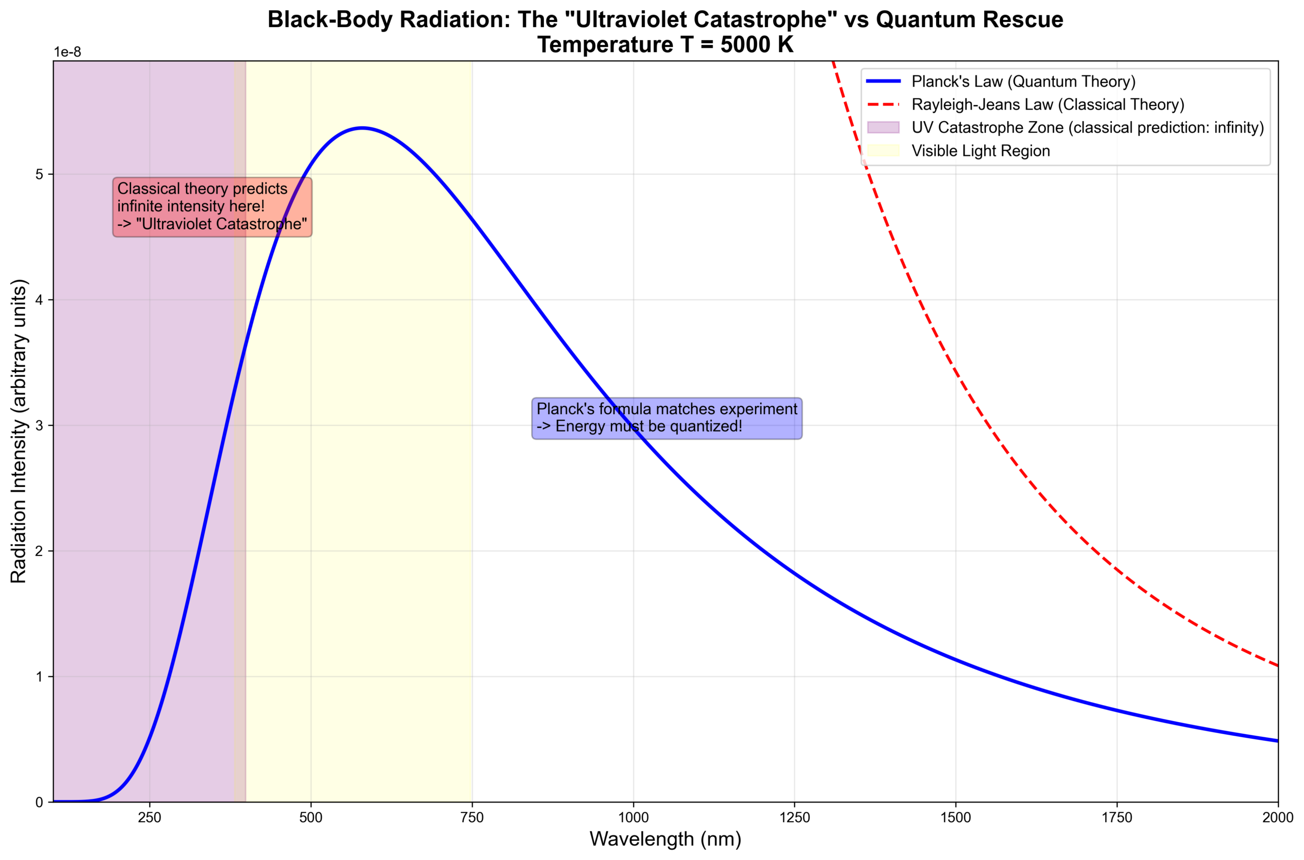
Cloud #1: The Black-Body Radiation Problem
Imagine a perfectly black object — one that absorbs all light that hits it, reflecting nothing. Now heat it up.
Experimental observations:
– At low temperatures, it glows red (infrared)
– At higher temperatures, it glows white (visible light)
– At even higher temperatures, it glows blue (ultraviolet)
This seems natural enough, right? Any blacksmith knows the progression: dark iron turns red, then orange, then yellow, then white-hot.
But here’s the question: what did classical physics predict?
According to classical theory (the Rayleigh-Jeans formula), energy should be distributed evenly across all frequencies. This implied that:
– A heated object would emit infinite amounts of ultraviolet light
– Its energy output would be infinite
This was called the “Ultraviolet Catastrophe.”
But experiments told a different story: there was no infinite energy. Heated objects did not explode into cosmic oblivion.
Classical physics had failed.
Cloud #2: The Michelson-Morley Experiment (1887)
Nineteenth-century physicists believed that light waves, like sound waves through air, needed a medium to travel through. They hypothesized that all of space was filled with a substance called the “luminiferous ether.”
In 1887, Albert Michelson and Edward Morley designed a precision experiment: Earth orbits the Sun at roughly 30 km/s. If the ether existed, we should be able to detect an “ether wind” — much like the wind you feel when you ride a bicycle.
The result: nothing. Absolutely nothing.
They improved the instrument’s sensitivity to 1/100th of Earth’s orbital velocity. Still nothing.
No ether? Then what does light travel through?
This puzzle led directly to Einstein’s special relativity in 1905, but that’s a story for another day.
Cloud #3: The Photoelectric Effect (1887)
Also in 1887, Hertz — while confirming the existence of electromagnetic waves — stumbled upon a peculiar phenomenon:
When ultraviolet light struck a metal surface, the metal ejected electrons. This became known as the photoelectric effect.
The strange part:
1. More intense light knocked out more electrons (that made sense)
2. But the energy of each electron depended only on the light’s frequency, not its intensity (that made no sense!)
3. Below a certain frequency threshold, no amount of light — however intense — could dislodge a single electron (that made even less sense!)
Classical theory said: light is a wave, and a wave’s energy depends on its amplitude (intensity). Brighter light should give each electron more energy.
But the experiments said: no.
Blinding red light couldn’t budge a single electron, yet a feeble beam of ultraviolet light knocked them out easily.
Classical theory had failed again.
Planck’s Reluctant Revolution
The Desperation of Black-Body Radiation
Planck was a classical physicist through and through. He believed in thermodynamics, trusted in the orderly nature of the universe, and was the kind of man who would argue about a decimal point for three days.
But the black-body radiation problem had held him hostage for six years.
He tried every classical approach:
– Electromagnetic theory — no luck
– Statistical mechanics — no luck
– The second law of thermodynamics — no luck
By October 1900, he gave up on deriving the answer from first principles and decided to simply “get the math right.” He fitted an empirical formula to the experimental data:
rho(v,T) = (8 pi h v³/c³) x 1/(e^(hv/kT) – 1)
The formula matched the experiments perfectly!
But the question was: what does it mean?
Planck stared at his formula for two months until a deeply unsettling realization crystallized: there was only one interpretation that worked.
Energy is not continuous. It comes in discrete packets.
Energy Quantization
Planck proposed that energy can only exist in multiples of a fundamental unit — a “quantum” (from the Latin quantus, meaning “how much”):
E = nhv
Where:
– n = 0, 1, 2, 3, … (integers only)
– h = 6.626×10⁻³⁴ J·s (Planck’s constant)
– v = frequency
This meant:
– You cannot have “half” a quantum of energy
– Energy is like a staircase, not a ramp
– There is a minimum unit: deltaE = hv
For ultraviolet light (high frequency), each quantum is large — it takes a lot of energy to “climb” to the next step, so radiation at those frequencies is suppressed.
For infrared light (low frequency), each quantum is small — easy to climb, so radiation flows freely.
This is why the Ultraviolet Catastrophe never happens in reality — high-frequency radiation is too “expensive” for the system to afford.
Planck’s Inner Struggle
But Planck himself didn’t truly believe his own hypothesis.
He regarded it as a “mathematical trick” — a stopgap measure to make the formula work. He spent the next decade trying to re-derive his result using purely classical reasoning.
He failed.
In 1931, Planck looked back on those years:
“My futile attempts to fit the quantum of action somehow into the classical theory continued for a number of years and cost me a great deal of effort. Some of my colleagues saw a tragic element in this. But I disagree, because the thorough exploration it gave me was of great value.”
He had lit the fuse of a revolution, then spent years trying to stamp out the flames.
Einstein’s Audacity
In 1905, a 26-year-old patent clerk changed everything.
The Light Quantum Hypothesis
Albert Einstein read Planck’s paper and took the idea further — much further.
Planck had said: the emission and absorption of energy is quantized, but light itself is still a wave.
Einstein said: no. Light itself is made of particles.
He proposed that light consists of discrete bundles of energy — “light quanta” (later renamed “photons”) — each carrying an energy of:
E = hv
Not nhv (many quanta). Just hv (one quantum at a time).
Photons are like bullets, striking the metal surface one by one.
Explaining the Photoelectric Effect
With the light quantum hypothesis, the photoelectric effect suddenly made perfect sense:
- Energy of a photon = hv
- The metal’s binding energy (work function) = W₀
- If hv < W₀, the photon doesn’t carry enough energy — no electron is ejected
- If hv > W₀, the surplus energy becomes the electron’s kinetic energy: KE = hv – W₀
Therefore:
– Frequency determines electron energy (each photon’s energy)
– Intensity determines electron count (number of photons)
Elegant and complete.
In 1921, Einstein received the Nobel Prize in Physics for “his explanation of the photoelectric effect.” Ironically, his far more famous theory of relativity was still too controversial for the Nobel committee, but the light quantum hypothesis had been confirmed beyond doubt.
Wave-Particle Duality
But this created a profound paradox:
Is light a wave, or a particle?
The double-slit experiment (Thomas Young, 1801) proved: light is a wave (it produces interference fringes).
The photoelectric effect proved: light is a particle (individual photons).
Both are correct.
This is wave-particle duality — one of the most bewildering discoveries of 20th-century physics.
Light is both wave and particle. Or more precisely: light transcends the very categories of “wave” and “particle” that our minds have constructed.
Python Analysis: Witnessing the Birth of the Quantum
Enough theory. Let’s use Python to recreate these historic discoveries.
Model 1: Black-Body Radiation — Visualizing the “Ultraviolet Catastrophe”
First, we need to define two formulas: Planck’s quantum formula and the classical Rayleigh-Jeans formula.
import numpy as np
import matplotlib.pyplot as plt
from scipy.constants import h, c, k

# Font configuration
plt.rcParams['font.sans-serif'] = ['Arial', 'Helvetica']
plt.rcParams['axes.unicode_minus'] = False

def planck_law(wavelength, T):
    """Planck's law (quantum theory)"""
    return (8 * np.pi * h * c / wavelength**5) / (np.exp(h * c / (wavelength * k * T)) - 1)

def rayleigh_jeans_law(wavelength, T):
    """Rayleigh-Jeans law (classical theory)"""
    return 8 * np.pi * k * T / wavelength**4
What’s the difference between these two formulas?
The classical Rayleigh-Jeans formula assumes energy can be subdivided infinitely — which leads to a prediction of infinite radiation intensity at short wavelengths (the ultraviolet region). Planck’s formula introduces the constraint of quantization: energy comes in discrete packets, and high-frequency radiation is too “expensive,” so the intensity doesn’t blow up to infinity.
Next, we set the temperature to 5000K (roughly the surface temperature of the Sun) and calculate predictions from both theories:
def visualize_blackbody_radiation():
    """Visualize black-body radiation: classical vs quantum"""

    wavelength_nm = np.linspace(100, 3000, 1000)
    wavelength_m = wavelength_nm * 1e-9
    T = 5000  # Approximate surface temperature of the Sun

    planck_intensity = planck_law(wavelength_m, T)
    rayleigh_intensity = rayleigh_jeans_law(wavelength_m, T)
Why 5000K? Because it’s close to the Sun’s surface temperature. Everyone sees the Sun every day, yet classical physics cannot explain why it doesn’t blow itself apart in a burst of ultraviolet radiation.
Now let’s plot the results:
    fig, ax = plt.subplots(figsize=(12, 8))

    # Quantum theory (blue solid line)
    ax.plot(wavelength_nm, planck_intensity * 1e-13,
            'b-', linewidth=2.5, label="Planck's Law (Quantum Theory)")

    # Classical theory (red dashed line) — only for long wavelengths; short wavelengths blow up
    mask = wavelength_nm > 500
    ax.plot(wavelength_nm[mask], rayleigh_intensity[mask] * 1e-13,
            'r--', linewidth=2, label='Rayleigh-Jeans Law (Classical Theory)')

    # Mark the ultraviolet catastrophe zone and visible light region
    uv_region = wavelength_nm < 400
    ax.fill_between(wavelength_nm[uv_region], 0,
                     np.max(planck_intensity * 1e-13) * 1.2,
                     alpha=0.2, color='purple',
                     label='UV Catastrophe Zone (classical prediction: infinity)')

    visible_region = (wavelength_nm >= 380) & (wavelength_nm <= 750)
    ax.fill_between(wavelength_nm[visible_region], 0,
                     np.max(planck_intensity * 1e-13) * 1.2,
                     alpha=0.1, color='yellow', label='Visible Light Region')
Notice the red dashed line — we only plotted it from 500 nm onward. If we extended it into the ultraviolet region, the curve would shoot toward infinity.
This is the Ultraviolet Catastrophe, rendered visible.
    ax.set_xlabel('Wavelength (nm)', fontsize=14)
    ax.set_ylabel('Radiation Intensity (arbitrary units)', fontsize=14)
    ax.set_title(f'Black-Body Radiation: The "Ultraviolet Catastrophe" vs Quantum Rescue\nTemperature T = {T} K',
                 fontsize=16, fontweight='bold')
    ax.legend(fontsize=12, loc='upper right')
    ax.grid(True, alpha=0.3)
    ax.set_xlim(100, 2000)
    ax.set_ylim(0, np.max(planck_intensity * 1e-13) * 1.1)

    ax.text(200, np.max(planck_intensity * 1e-13) * 0.9,
            'Classical theory predicts\ninfinite intensity here!\n-> "Ultraviolet Catastrophe"',
            fontsize=11, bbox=dict(boxstyle='round', facecolor='red', alpha=0.3))

    ax.text(800, np.max(planck_intensity * 1e-13) * 0.6,
            "Planck's formula matches experiment\n-> Energy must be quantized!",
            fontsize=11, bbox=dict(boxstyle='round', facecolor='blue', alpha=0.3))

    plt.tight_layout()
    plt.savefig('blackbody_radiation.png', dpi=300, bbox_inches='tight')
    plt.show()
Finally, we verify some specific numbers using Wien’s displacement law and the Stefan-Boltzmann law:
    peak_wavelength = 2.898e-3 / T
    print(f"\n[Wien's Displacement Law]")
    print(f"Temperature T = {T} K")
    print(f"Peak wavelength lambda_max = {peak_wavelength*1e9:.1f} nm")

    stefan_boltzmann = 5.67e-8
    total_power = stefan_boltzmann * T**4
    print(f"\n[Stefan-Boltzmann Law]")
    print(f"Total radiated power proportional to T^4 = {total_power:.2e} W/m2")

# Run
visualize_blackbody_radiation()
What does this analysis reveal?
The blue curve (Planck) perfectly describes the experimental data. The red curve (classical) is roughly acceptable at long wavelengths, but falls apart completely in the ultraviolet.
Without quantization, the universe would explode in ultraviolet radiation.
The grand edifice of classical physics was pierced by a single curve.
Model 2: The Photoelectric Effect — Einstein’s Light Quanta
Next, we simulate the photoelectric effect. We begin by defining the work functions (binding energies) for five metals:
def photoelectric_effect_simulation():
    """Photoelectric effect simulation"""

    metals = {
        'Sodium (Na)': 2.28,
        'Aluminum (Al)': 4.08,
        'Copper (Cu)': 4.70,
        'Zinc (Zn)': 4.31,
        'Silver (Ag)': 4.73
    }

    wavelengths = np.linspace(200, 600, 100)
    frequencies = c / (wavelengths * 1e-9)
    photon_energies = h * frequencies / 1.6e-19  # Convert to eV
What is a work function?
Different metals bind their electrons with different strengths. Sodium only needs 2.28 eV to release an electron; silver needs 4.73 eV. A photon’s energy must exceed the work function to knock an electron free.
This is why even blindingly intense red light can’t eject electrons from copper — each individual photon simply doesn’t carry enough energy.
Now we plot two graphs that expose the core paradox of the photoelectric effect:
    fig, (ax1, ax2) = plt.subplots(1, 2, figsize=(16, 6))

    # Left plot: Cutoff frequencies for different metals
    colors = ['blue', 'green', 'red', 'orange', 'purple']

    for (metal, work_function), color in zip(metals.items(), colors):
        kinetic_energy = photon_energies - work_function
        kinetic_energy[kinetic_energy < 0] = 0

        ax1.plot(wavelengths, kinetic_energy,
                linewidth=2, label=f'{metal} (W0={work_function} eV)', color=color)

        cutoff_wavelength = h * c / (work_function * 1.6e-19) * 1e9
        ax1.axvline(cutoff_wavelength, color=color, linestyle='--', alpha=0.5)
        ax1.text(cutoff_wavelength, 5, f'{cutoff_wavelength:.0f}nm',
                rotation=90, va='bottom', fontsize=9, color=color)

    ax1.set_xlabel('Wavelength of Light (nm)', fontsize=13)
    ax1.set_ylabel('Photoelectron Kinetic Energy (eV)', fontsize=13)
    ax1.set_title('Photoelectric Effect: Frequency Determines Electron Energy\nKE = hv - W0',
                  fontsize=14, fontweight='bold')
    ax1.legend(fontsize=10, loc='upper right')
    ax1.grid(True, alpha=0.3)
    ax1.set_xlim(200, 600)
    ax1.set_ylim(0, 6)
    ax1.axvspan(380, 750, alpha=0.1, color='yellow', label='Visible Light')
The left plot makes it clear: every metal has its own “cutoff wavelength.” If the wavelength is too long (frequency too low), the photon doesn’t carry enough energy, and the curve drops to zero.
Classical theory simply cannot account for this. If light is a wave, why can’t intense light eject electrons?
    # Right plot: Light intensity vs number of electrons (not energy)
    intensities = np.array([1, 2, 5, 10])
    wavelength_fixed = 300  # nm
    photon_energy_fixed = h * c / (wavelength_fixed * 1e-9) / 1.6e-19

    work_function_Na = metals['Sodium (Na)']

    if photon_energy_fixed > work_function_Na:
        electron_counts = intensities * 100
        electron_energy = photon_energy_fixed - work_function_Na

        bars = ax2.bar(intensities, electron_counts, width=0.8,
                      color='skyblue', edgecolor='navy', linewidth=2)

        for bar, count in zip(bars, electron_counts):
            ax2.text(bar.get_x() + bar.get_width()/2, bar.get_height() + 10,
                    f'{int(count)} electrons\neach at {electron_energy:.2f} eV',
                    ha='center', fontsize=10,
                    bbox=dict(boxstyle='round', facecolor='yellow', alpha=0.5))

    ax2.set_xlabel('Light Intensity (relative)', fontsize=13)
    ax2.set_ylabel('Number of Ejected Electrons', fontsize=13)
    ax2.set_title(f'Photoelectric Effect: Intensity Controls Electron Count (Not Energy)\nMetal: Sodium, Wavelength: {wavelength_fixed} nm',
                  fontsize=14, fontweight='bold')
    ax2.grid(True, alpha=0.3, axis='y')

    ax2.text(6, 800,
            'Key Insight:\n'
            'Higher intensity -> more electrons\n'
            'But each electron has the SAME energy!\n'
            'Electron energy depends only on frequency\n\n'
            'Classical wave theory cannot explain this!\n'
            '-> Light must be particles (photons)',
            fontsize=11, bbox=dict(boxstyle='round', facecolor='lightblue', alpha=0.7))

    plt.tight_layout()
    plt.savefig('photoelectric_effect.png', dpi=300, bbox_inches='tight')
    plt.show()
The right plot reveals another crucial finding: increase the light intensity tenfold, and you get ten times as many ejected electrons — but every single electron carries the same energy!
If light were purely a wave, brighter light should give each electron more energy. But the experiments say otherwise.
Photons behave like bullets, striking the metal one at a time. Intensity determines how many bullets there are; frequency determines how powerful each bullet is.
Finally, let’s run a virtual laboratory to verify:
    print("\n" + "="*60)
    print("[Photoelectric Effect Virtual Lab]")
    print("="*60)

    chosen_metal = 'Zinc (Zn)'
    work_function = metals[chosen_metal]
    print(f"\nSelected: {chosen_metal}")
    print(f"Work function W0 = {work_function} eV")
    print(f"Cutoff wavelength lambda_0 = {h * c / (work_function * 1.6e-19) * 1e9:.1f} nm")

    test_wavelengths = [200, 300, 400, 500]
    print("\nExperimental Results:")
    print("-" * 60)
    print(f"{'Wavelength(nm)':<16} {'Photon E (eV)':<16} {'Electron KE(eV)':<16} {'Result'}")
    print("-" * 60)

    for wl in test_wavelengths:
        photon_e = h * c / (wl * 1e-9) / 1.6e-19
        ke = photon_e - work_function
        if ke > 0:
            result = "Electron ejected!"
        else:
            result = "No ejection"
        print(f"{wl:<16} {photon_e:<16.2f} {max(0, ke):<16.2f} {result}")

# Run
photoelectric_effect_simulation()
Output:
Selected: Zinc (Zn)
Work function W0 = 4.31 eV
Cutoff wavelength lambda_0 = 287.7 nm

Wavelength(nm)   Photon E (eV)    Electron KE(eV)  Result
------------------------------------------------------------
200              6.20             1.89             Electron ejected!
300              4.14             0.00             No ejection
400              3.10             0.00             No ejection
500              2.48             0.00             No ejection
See the pattern? Zinc’s cutoff wavelength is 287.7 nm. Only 200 nm deep-ultraviolet light can knock out an electron; everything above 300 nm is completely ineffective.
This is how the quantum world works: energy is discrete, not continuous.
Model 3: The Death of Determinism — From Newton to Heisenberg
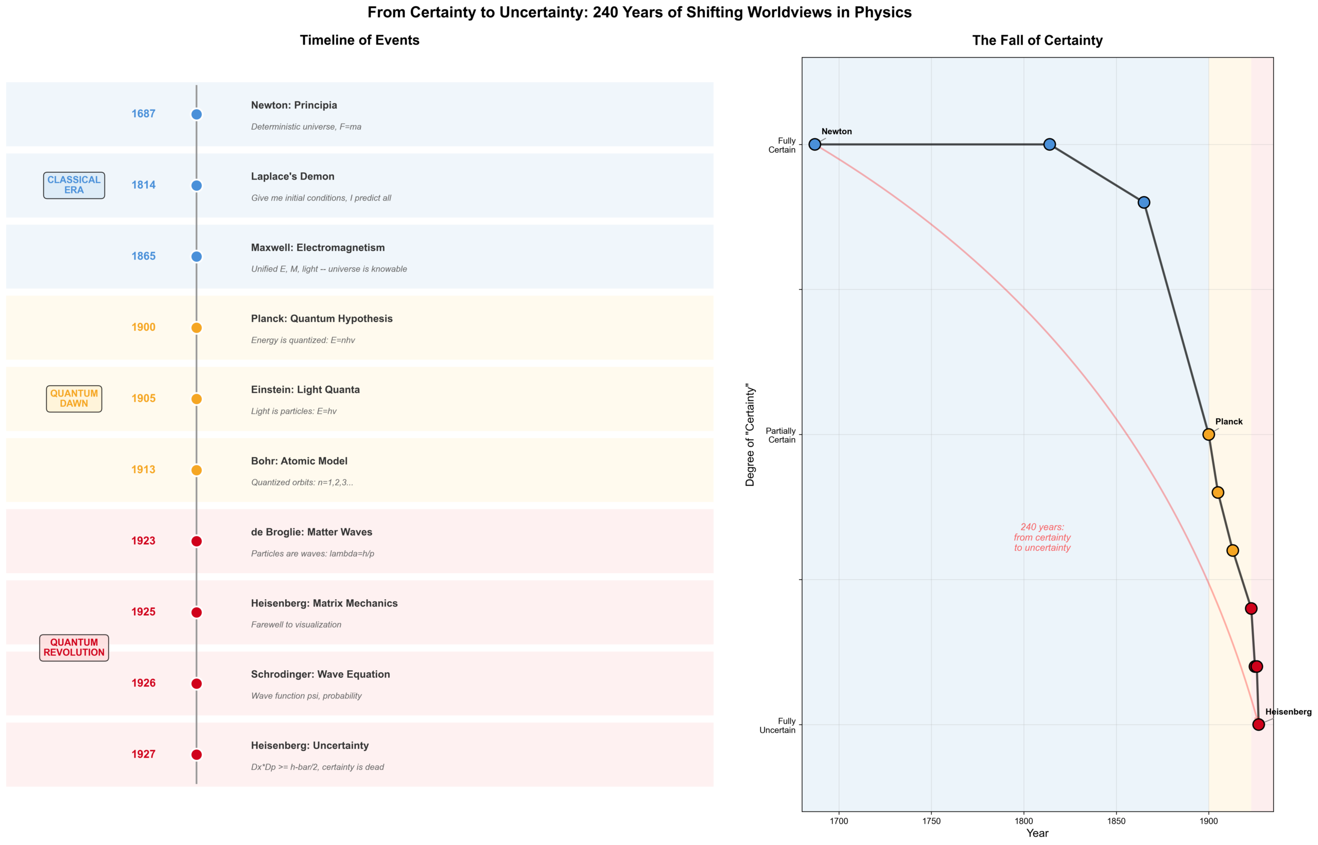
Finally, let’s create a single visualization tracing the 240-year evolution of physics’ worldview.
We start by plotting key events on a timeline:
def determinism_timeline():
    """Visualize the transformation of physics' worldview"""

    fig, ax = plt.subplots(figsize=(14, 10))

    events = [
        (1687, "Newton\nPrincipia", "Deterministic universe\nF=ma", 'blue', 1.0),
        (1814, "Laplace's\nDemon", "Give me initial conditions\nI know everything", 'blue', 1.0),
        (1865, "Maxwell\nElectromagnetics", "Unified E, M, light\nUniverse is knowable", 'blue', 0.9),
        (1900, "Planck\nQuantum Hypothesis", "Energy is quantized\nE=nhv", 'orange', 0.5),
        (1905, "Einstein\nLight Quanta", "Light is particles\nE=hv", 'orange', 0.4),
        (1913, "Bohr\nAtomic Model", "Quantized electron orbits\nn=1,2,3...", 'orange', 0.3),
        (1923, "de Broglie\nMatter Waves", "Particles are waves too\nlambda=h/p", 'red', 0.2),
        (1925, "Heisenberg\nMatrix Mechanics", "Farewell to visualization\nEverything is matrices", 'red', 0.1),
        (1926, "Schrodinger\nWave Mechanics", "Wave function psi\nProbability interpretation", 'red', 0.1),
        (1927, "Heisenberg\nUncertainty Principle", "Dx*Dp >= h-bar/2\nCertainty is dead", 'red', 0.0)
    ]
Ten events spanning 240 years. Each event carries a “certainty index” — from 1.0 (complete certainty) to 0.0 (fundamental uncertainty).
Notice something striking: during the 213 years from 1687 to 1900, the certainty index dropped by only 0.1. But in the 27 years from 1900 to 1927, it plummeted by 0.5.
The quantum revolution moved faster than anyone could have imagined.
    years = [e[0] for e in events]
    certainties = [e[4] for e in events]

    # Background gradient: blue -> orange -> red
    for i in range(len(events)-1):
        ax.fill_between([events[i][0], events[i+1][0]], 0, 1,
                        alpha=0.3, color=events[i][3])

    # Certainty curve
    ax.plot(years, certainties, 'k-', linewidth=3, label='"Certainty" Index')
    ax.scatter(years, certainties, c=[e[3] for e in events],
              s=300, edgecolor='black', linewidth=2, zorder=5)

    # Annotate events
    for year, person, description, color, certainty in events:
        ax.text(year, certainty + 0.1, person,
               ha='center', fontsize=10, fontweight='bold')
        ax.text(year, certainty - 0.15, description,
               ha='center', fontsize=8, style='italic',
               bbox=dict(boxstyle='round', facecolor=color, alpha=0.3))

    # Three eras
    ax.text(1750, 0.95, 'Classical Era\n"The universe is a clock"',
           fontsize=14, ha='center', fontweight='bold',
           bbox=dict(boxstyle='round', facecolor='lightblue', alpha=0.5))
    ax.text(1910, 0.45, 'Quantum Dawn\n"Energy is discrete"',
           fontsize=14, ha='center', fontweight='bold',
           bbox=dict(boxstyle='round', facecolor='lightyellow', alpha=0.5))
    ax.text(1926, 0.05, 'Quantum Revolution\n"Uncertainty is fundamental"',
           fontsize=14, ha='center', fontweight='bold',
           bbox=dict(boxstyle='round', facecolor='lightcoral', alpha=0.5))

    ax.set_xlim(1680, 1935)
    ax.set_ylim(-0.2, 1.15)
    ax.set_xlabel('Year', fontsize=14)
    ax.set_ylabel('Degree of "Certainty"', fontsize=14)
    ax.set_title('From Certainty to Uncertainty: 240 Years of Shifting Worldviews in Physics',
                fontsize=16, fontweight='bold')
    ax.grid(True, alpha=0.3)
    ax.legend(fontsize=12, loc='upper right')
    ax.set_yticks([0, 0.5, 1.0])
    ax.set_yticklabels(['Fully Uncertain\n(Quantum World)', 'Partially Certain\n(Transitional)', 'Fully Certain\n(Classical World)'])

    plt.tight_layout()
    plt.savefig('determinism_timeline.png', dpi=300, bbox_inches='tight')
    plt.show()
This chart transitions from blue (certainty) to red (uncertainty), giving visual form to humanity’s radical shift in understanding the cosmos.
Finally, let’s compare the worldviews of three eras side by side:
    print("\n" + "="*70)
    print("[Three Worldviews in Physics]")
    print("="*70)

    worldviews = [
        {'Era': 'Classical (1687-1900)', 'Key Figures': 'Newton, Laplace',
         'Core Belief': 'Determinism', 'Universe Metaphor': 'Precision clockwork',
         'Causality': 'Past determines future', 'Free Will': 'An illusion (all is predetermined)',
         'Role of God': 'The Prime Mover'},
        {'Era': 'Quantum Dawn (1900-1925)', 'Key Figures': 'Planck, Einstein',
         'Core Belief': 'Energy is discontinuous', 'Universe Metaphor': 'A glitching clock',
         'Causality': 'Still causal, but with limits', 'Free Will': 'Uncertain',
         'Role of God': '"Does not play dice" (Einstein insisted)'},
        {'Era': 'Quantum Revolution (1925-present)', 'Key Figures': 'Heisenberg, Schrodinger, Bohr',
         'Core Belief': 'Fundamental uncertainty', 'Universe Metaphor': 'A probability cloud',
         'Causality': 'Only probabilities, no certainties', 'Free Will': 'Possibly real (room exists)',
         'Role of God': '"Does play dice" (Bohr)'}
    ]

    for wv in worldviews:
        print(f"\n[{wv['Era']}]")
        for key, value in wv.items():
            if key != 'Era':
                print(f"  {key:<18}: {value}")

# Run
determinism_timeline()
What does this analysis reveal?
1814: “Give me the initial conditions, and I will know everything.”
1927: “You can never simultaneously know both position and momentum.”
In just 113 years, humanity fell from “omniscience” to “fundamental unknowability.”
This was not merely a change in physics. It was the collapse of an entire worldview. And this collapse, as it turns out, resonates in astonishing ways with insights that Eastern philosophers articulated over two thousand years earlier.
Echoes from Eastern Philosophy
“The Tao That Can Be Told Is Not the Eternal Tao”
When Planck, in desperation, introduced energy quanta; when Einstein declared “light is both particle and wave”; when Heisenberg discovered that “uncertainty is fundamental” — they were, in essence, saying:
Our descriptions of the world can never fully capture the world itself.
This calls to mind the opening lines of the Tao Te Ching, written by the Chinese sage Laozi (Lao Tzu) around the 4th century BCE. It is one of the most influential philosophical texts ever written — a slim collection of 81 verses that has shaped Chinese thought for over two millennia. Its central concept, the Tao (literally “the Way”), refers to the fundamental, indescribable principle underlying all of reality:
“The Tao that can be told is not the eternal Tao;
the name that can be named is not the eternal name.”
In other words: any reality that can be pinned down in language is, by that very act, no longer the full reality. The moment you label something, you limit it — a concept that resists the very definitions we try to impose on it, which is precisely why quantum physicists have found it so resonant.
Quantum mechanics says: a particle has no definite state before measurement.
Laozi says: the Tao has no fixed form before it is named.
Quantum mechanics says: observation alters reality.
Laozi says: “When all the world knows beauty as beauty, ugliness arises.” The act of defining one thing simultaneously creates its opposite.
“Being and Non-Being Create Each Other”
Laozi also wrote:
“Being and non-being create each other,
difficult and easy complement each other,
long and short define each other,
high and low depend on each other.”
Doesn’t wave-particle duality work in exactly this way?
– Observe the “wave,” and you lose the “particle”
– Observe the “particle,” and you lose the “wave”
– The two are complementary — neither alone tells the whole story
Niels Bohr, the architect of the Copenhagen Interpretation of quantum mechanics, was deeply influenced by Eastern philosophy. In 1947, when he was awarded Denmark’s highest honor (the Order of the Elephant), he chose a personal coat of arms. Its central image?
The yin-yang symbol (taijitu).
The Latin inscription on his coat of arms read: Contraria sunt complementa — “Opposites are complementary.”
Preview: What’s Next
It took quantum mechanics 25 years to convince Western scientists that “the world is not deterministic.”
But 2,500 years earlier, Eastern thinkers had been saying things like:
- “Form is emptiness, emptiness is form” (Heart Sutra — a foundational Buddhist text teaching that all phenomena lack inherent, independent existence)
- “The ten thousand things flourish and then each returns to the root” (Tao Te Ching — Laozi’s observation that all things arise and dissolve back into their source)
- “In dreams we clearly perceive the six realms of existence; after awakening, the universe is empty” (Song of Enlightenment by Yongjia Xuanjue, a Zen master, expressing the idea that our ordinary perception of reality is itself dreamlike)
What did they see?
In the next article, we’ll explore what happens when quantum mechanics’ Copenhagen Interpretation meets the Kyoto School of Zen philosophy.
Closing Reflections: The Cost of Revolution
In 1918, Planck was awarded the Nobel Prize. The citation honored “his discovery of energy quanta, which opened a new era in physics.”
But Planck’s feelings were complicated. He had lit the fuse of a revolution, yet he was never entirely sure it was the right thing to do.
By 1931, when Planck was 73, a younger generation of physicists had constructed the full edifice of quantum mechanics — matrix mechanics, wave mechanics, the uncertainty principle, the probability interpretation.
These theories had thoroughly demolished the classical worldview he held dear.
Someone asked Planck: “Do you regret proposing the quantum hypothesis?”
He replied:
“A new scientific truth does not triumph by convincing its opponents and making them see the light, but rather because its opponents eventually die, and a new generation grows up that is familiar with it.”
It’s a bittersweet remark, but it speaks a deeper truth: revolutions are always painful — especially for the revolutionaries themselves.
Planck had opened Pandora’s box.
In the 25 years that followed (1900–1925), physicists would discover that:
– Electrons “jump” rather than move continuously
– Particles can be in two places at once
– Measurement “creates” reality
– The observer cannot be separated from the world
Newton’s universe — that grand, deterministic, predictable palace — was crumbling.
And from its ruins, a stranger, more mysterious, and more profound universe would emerge.
Next Article Preview
Episode 2: The Copenhagen Interpretation vs. The Kyoto School — A Dialogue Between Two Wisdoms
1954, Copenhagen.
Niels Bohr, one of the founding fathers of quantum mechanics, sat across from D.T. Suzuki, the Japanese Zen scholar who did more than anyone to introduce Zen Buddhism to the West.
Bohr pointed to the yin-yang symbol on his wall and said: “It took me thirty years to understand complementarity. Your ancestors understood it two thousand years ago.”
Suzuki smiled and replied: “No — we did not understand it. We are it.”
In the next episode, we’ll explore:
– What does the Copenhagen Interpretation actually say?
– What does it mean that “observation creates reality”?
– Why did Bohr choose the yin-yang symbol for his coat of arms?
– What deep connections exist between quantum mechanics and Zen?
Two ways of seeking truth, separated by two thousand years — converging on one stunning conclusion.
References
- Planck, M. (1900). “On the Theory of the Energy Distribution Law of the Normal Spectrum”. Verhandlungen der Deutschen Physikalischen Gesellschaft.
- Einstein, A. (1905). “On a Heuristic Point of View Concerning the Production and Transformation of Light”. Annalen der Physik.
- Kragh, H. (2000). Max Planck: The reluctant revolutionary. Physics World.
- Laozi (4th century BCE). Tao Te Ching. (Translations by Stephen Mitchell, D.C. Lau, and others.)
- Capra, F. (1975). The Tao of Physics. Shambhala.
- Pais, A. (1982). Subtle is the Lord: The Science and the Life of Albert Einstein. Oxford University Press.